“Can we fine-tune the 7B model on our support tickets?” sounds like a one-line request. Then you do the maths: 7 billion numbers inside the model (its “weights”), each needing extra memory while it trains, and the answer is roughly 108 GB of GPU memory.
LoRA is the reason that answer changed. LoRA fine-tuning (Low-Rank Adaptation, Hu et al., 2021) freezes the whole pre-trained model and trains two thin matrices next to each weight matrix instead. On GPT-3 175B, the paper reported 10,000× fewer trainable parameters and 3× less GPU memory than full fine-tuning, with no extra inference latency. Today LoRA fine-tuning is the default way most teams adapt open models.
📌 TL;DR
- What LoRA does: it fine-tunes a big model by freezing it and training two small matrices next to each layer. That’s often under 1% of the parameters and about 14 GB of GPU memory instead of 108 GB for a 7B model, with no extra cost at inference once merged.
- Yes, this is a long read, on purpose. We build LoRA from zero with one cat-and-dog example, so along the way you’ll also pick up the ML basics it rests on: vectors, layers, attention, transformers, rank, SVD, gradients and training.
- It’s worth it if you want to understand LoRA, not just call it. Every later topic (QLoRA, choosing a rank, merging, serving) becomes easy once the basics click.
- Short on time? Read the “In a hurry?” box below, then use the “How to read this post” links to jump to what you need.
This one is personal for me. I spend most of my time on the data side: pipelines, Spark tuning, table layouts. LoRA stopped being theory for me when I was retraining a DeBERTa model for prompt-injection detection: a classifier that has to keep up with new attack patterns, so it gets retrained again and again.
Implementing LoRA fine-tuning there is what made me really understand it: freeze the big pre-trained model, train a small LoRA adapter for the new data, keep each version as a small file, and retrain in a fraction of the time and memory. Like most good engineering ideas, it’s about not doing work you don’t need to do. (If you read my post on Hilbert clustering in Iceberg, it’s the same spirit: skip what doesn’t matter.)
So let’s build low-rank adaptation from zero, for everyone. We’ll use one tiny example all the way through: a cat and a dog. With it, every idea (a layer, a weight change, rank, the LoRA formula, training, merging, serving) becomes a few numbers you can check by hand. Then we’ll scale the same ideas up to real models, with the exact formulas an ML engineer uses and a real experiment. No maths beyond multiplying and adding numbers is assumed; every symbol is explained the first time it appears.
By the end you’ll be able to:
- explain what fine-tuning changes inside a model, and why that change is “low-rank”;
- write down LoRA’s forward pass, initialization and gradients, and explain every symbol;
- compute how many parameters and how much memory LoRA saves for any layer;
- choose the LoRA rank, alpha, learning rate and target modules with reasons, not folklore;
- merge a LoRA adapter for zero-latency inference, or serve many adapters on one GPU.
IN A HURRY? THE WHOLE STORY IN FIVE LINES
- The idea: fine-tuning learns a weight change ΔW. LoRA bets that ΔW is low-rank (a few simple patterns explain it) and learns it as ΔW = B·A, two thin matrices, while W stays frozen.
- The formula: h = Wx + (α/r)·B(Ax). A starts random, B starts at zero, so at step 0 the model is exactly the original.
- The savings: a 4096 × 4096 layer goes from 16.8M trainable numbers to 65K at r = 8 (0.39%). A whole 7B model at r = 16 trains ~40M parameters (~0.6%), and memory drops from ~108 GB to ~14 GB (~4 GB with QLoRA).
- The recipe: LoRA rank r = 16–64, α = 2r, all linear layers, learning rate 1e-4 to 3e-4 (about 10× full fine-tuning).
- Deployment: merge W′ = W + (α/r)·BA for zero extra latency, or keep adapters separate and serve many fine-tunes on one base model (vLLM
enable_lora).
🧭 HOW TO READ THIS POST
- New to ML? Start at how a model computes. Everything builds on one cat-and-dog example.
- Know transformers? Jump to what fine-tuning changes or straight to what “low-rank” means.
- Want the LoRA maths? How LoRA fine-tuning works: the formula, α/r and why B starts at zero.
- Need a recipe? Setting up LoRA in practice, then the code.
- Deploying? Merging and serving adapters.
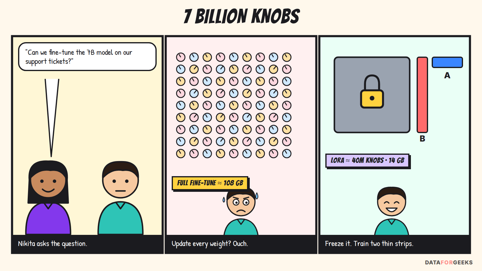
Table of Contents
How a model computes: the cat and dog example
Before we can change a model, we need to see what it computes. One tiny example carries us through the whole post.
Words become numbers
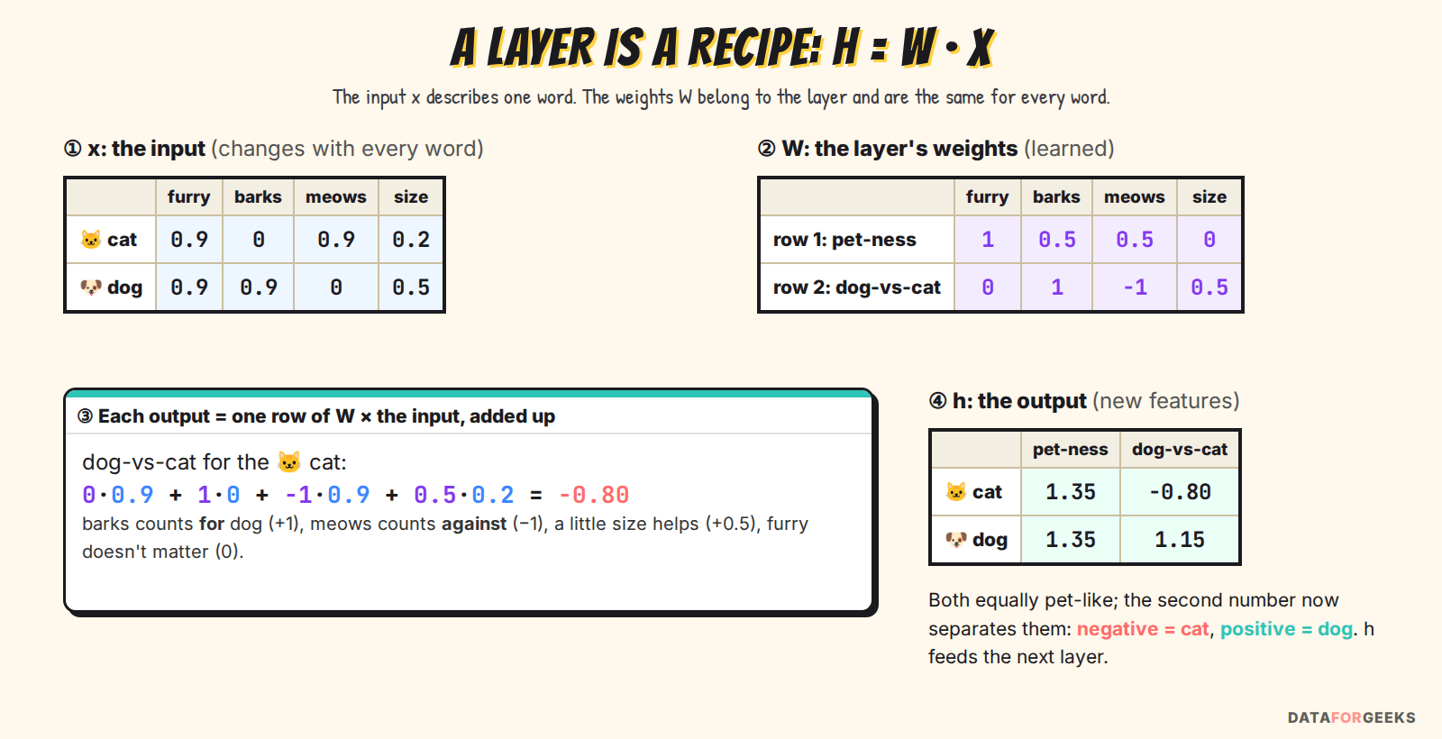
A model can’t read words. It turns each word into a vector: a list of numbers that describes it. Real models use thousands of numbers per word (strictly, per token: a word or a piece of one), and nobody can read them directly. To see the idea, let’s pretend there are just four, with human meanings:
| furry | barks | meows | size | |
|---|---|---|---|---|
| 🐱 cat | 0.9 | 0.0 | 0.9 | 0.2 |
| 🐶 dog | 0.9 | 0.9 | 0.0 | 0.5 |
This is the input, written x. It changes with every word the model reads.
A layer is a recipe: h = W x
A linear layer is a grid of learned numbers, W, that turns an input vector into an output vector: each output number is a weighted sum of the inputs.
Think of it as ingredients and a recipe. The input x holds the ingredients. W is the recipe: how much of each ingredient to use. Say our layer makes two new features, so W has 2 rows (one per output) and 4 columns (one per input):
| furry | barks | meows | size | This row computes… | |
|---|---|---|---|---|---|
| row 1 | 1 | 0.5 | 0.5 | 0 | “pet-ness” |
| row 2 | 0 | 1 | −1 | 0.5 | “dog-vs-cat” (+ dog, − cat) |
These are two different tables. The first describes an animal. This one belongs to the layer, and the same W is used for every word.
Now multiply. For the cat:
- pet-ness = 1·0.9 + 0.5·0.0 + 0.5·0.9 + 0·0.2 = 1.35
- dog-vs-cat = 0·0.9 + 1·0.0 + (−1)·0.9 + 0.5·0.2 = −0.80
For the dog:
- pet-ness = 1·0.9 + 0.5·0.9 + 0.5·0.0 + 0·0.5 = 1.35
- dog-vs-cat = 0·0.9 + 1·0.9 + (−1)·0.0 + 0.5·0.5 = +1.15
So hcat = [1.35, −0.80] and hdog = [1.35, 1.15]. Both are equally pet-like, and the second number now cleanly separates them. That output h becomes the input to the next layer, which mixes the features again, and so on through dozens of layers until the model makes a prediction.
YOU MIGHT BE WONDERING
Who picks the numbers in W?
Nobody. I picked these by hand so each row is easy to read. In a real model, W starts as random numbers. Training shows the model millions of examples, and each time it’s wrong, gradient descent nudges every weight slightly in the direction that makes it less wrong. The weights slowly settle into useful recipes like “barks → dog”. Those learned numbers are the model’s parameters; a 7B model has about 7 billion of them.
Also, real features don’t have neat labels like “furry”. The model invents its own, spread across many dimensions. The arithmetic is exactly the same.
From the toy to a real model
Written generally, a linear layer is:
Read ℝdout × din as “a grid of real numbers with dout rows and din columns”. In our toy, din = 4 and dout = 2, so W has 8 numbers. In a real model, each word is described by thousands of numbers (4,096 in Llama 2 7B), so a single recipe W can be 4096 × 4096: 16,777,216 numbers. (Many layers also add a bias vector, h = Wx + b. LoRA leaves it frozen too, so we’ll ignore it.)
Inside a real transformer: where the weight matrices live
Our pet recipe is one small layer. A real language model is a transformer: thousands of recipes like it, arranged in a fixed pattern. (Already know transformers? Skip to what fine-tuning changes.)
What is a transformer?
A transformer is the neural-network design behind almost every modern language model, including GPT, Llama, Claude, BERT and DeBERTa. It turns a sentence into vectors and refines them through a stack of identical blocks, each made of attention and an MLP. It was introduced in the 2017 paper “Attention Is All You Need”.
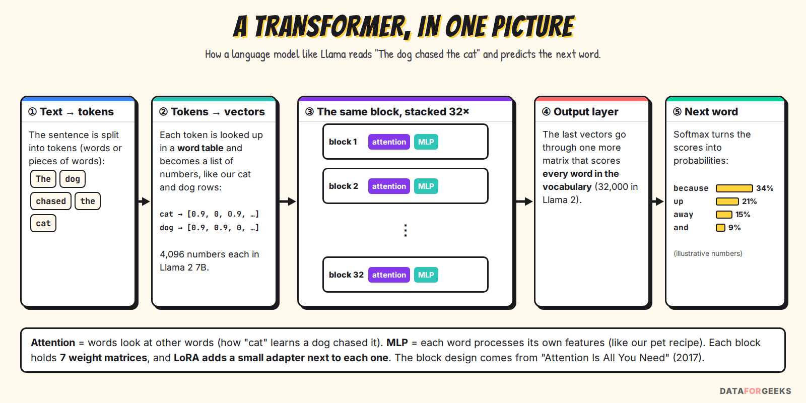
Here’s what happens when a model like Llama reads “The dog chased the cat” and predicts the next word:
- Text → tokens. The sentence is split into tokens: words or pieces of words.
- Tokens → vectors. Each token is looked up in a word table (the “embeddings”) and becomes a list of numbers, just like our cat and dog rows, only with 4,096 numbers instead of 4.
- The blocks. The vectors pass through a stack of identical blocks, 32 in Llama 2 7B. Each block has two parts: attention, where words look at other words, and an MLP, where each word processes its own features. Every block refines the vectors a little.
- Output layer. One last matrix scores every word in the vocabulary (32,000 in Llama 2).
- Next word. A softmax turns those scores into probabilities, and the model picks a likely next word, say “because”. Then it repeats, one word at a time.
Classifiers like the DeBERTa prompt-injection model from the start of this post use the same blocks. The only difference is the last step: instead of predicting the next word, a small classification head outputs a label, such as “injection” or “safe”.
For LoRA, one fact matters most: almost all of a transformer’s parameters live in the weight matrices inside the blocks. Let’s open one block with our pets.
Attention: recipes for looking at other words
An attention layer lets each word pull in information from the other words in the sentence. It does this with four weight matrices, each just a recipe like W: Wq (query), Wk (key), Wv (value) and Wo (output).
Take the sentence “The dog chased the cat.” The word “cat” on its own doesn’t know it was chased. Attention fixes that, in four small steps:
- Query, “what am I looking for?” Our toy Wq is [0, 0, 1, 0]: “if I meow, I’m looking for something that barks”. For the cat: q = 0.9. For the dog: q = 0.
- Key, “what do I offer?” Our toy Wk is [0, 1, 0, 0]: “I advertise how much I bark”. For the dog: k = 0.9. For the cat: k = 0.
- Score = query × key. Cat → dog: 0.9 × 0.9 = 0.81. Cat → cat: 0.9 × 0 = 0. A softmax turns scores into shares that add up to 100%: the cat pays 69% of its attention to the dog.
- Value and output. Wv decides what each word passes on (say, the dog’s size), and Wo mixes what the cat gathered back into its own features. The cat’s vector now carries “a dog chased me”.
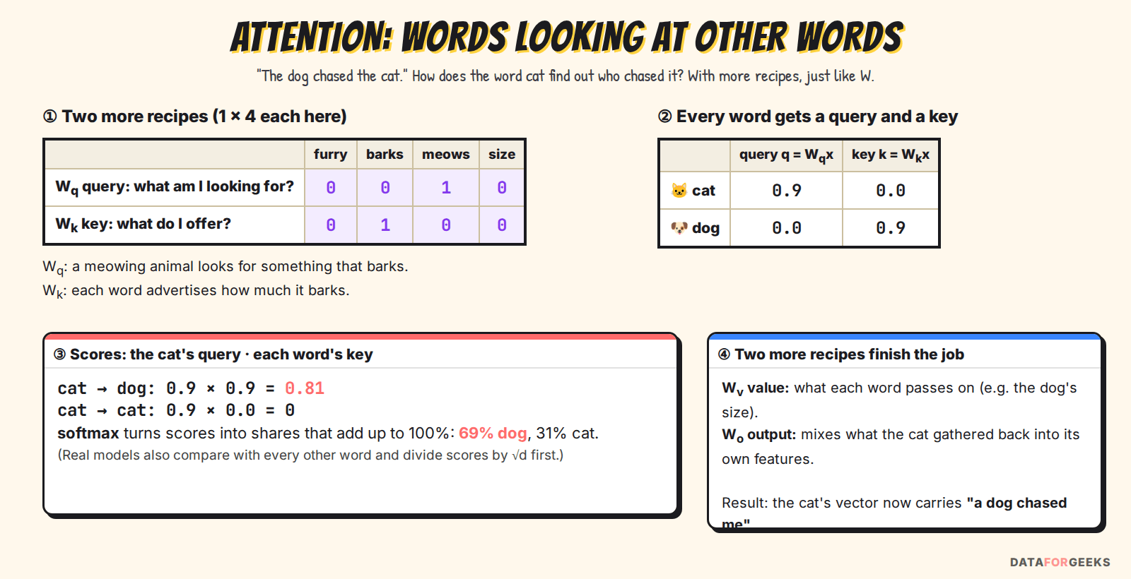
Real attention compares every word with every other word, uses many numbers per query and key instead of one, and divides scores by √d before the softmax. But the part that matters for LoRA fine-tuning is simple: Wq, Wk, Wv and Wo are four ordinary weight matrices, exactly like our pet recipe. In code they’re called q_proj, k_proj, v_proj and o_proj.
The MLP: recipes that work on each word
After attention, each word also goes through an MLP (a “feed-forward” layer): three more recipes, called gate_proj, up_proj and down_proj, that transform each word’s features on their own. Our pet recipe W, turning furry/barks/meows/size into pet-ness and dog-vs-cat, is exactly this kind of layer.
Why a 7B model has hundreds of these matrices
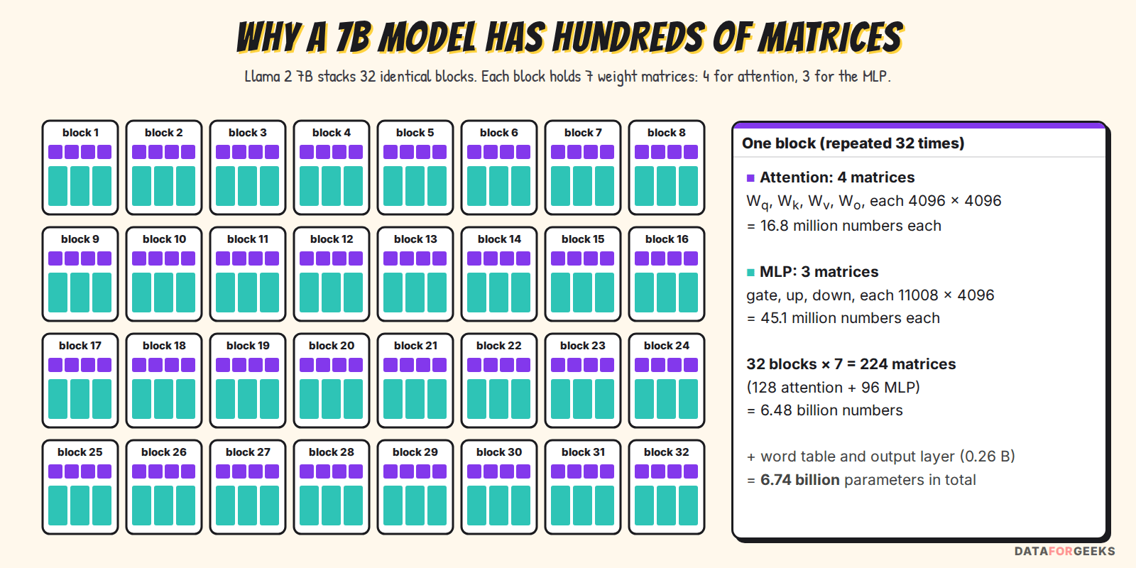
A transformer stacks the same block (attention + MLP) many times. Llama 2 7B has 32 blocks (why?), and each block holds 7 weight matrices:
- 4 attention matrices (Wq, Wk, Wv, Wo), each 4096 × 4096 = 16.8 million numbers;
- 3 MLP matrices (gate, up, down), each 11008 × 4096 = 45.1 million numbers.
32 blocks × 7 = 224 matrices: 128 attention and 96 MLP, holding 6.48 billion numbers. The word table and the output layer add 0.26 billion more, which gives the model’s 6.74 billion parameters. That’s why full fine-tuning is expensive: every one of those 224 matrices has its own W to change. LoRA fine-tuning instead gives each of them a tiny LoRA adapter. When this post says “layer”, it means one of these 224 matrices, not a whole block.
Why stack the same block 32 times?
One block can do only one round of “look at the other words, then think”. Stacking blocks lets the model do many rounds, and each round builds on what the previous ones worked out.
First, a clarification: “the same block” means the same design, not the same numbers. All 32 blocks have the same layout (attention + MLP, 7 matrices), but every block has its own weights. Block 1’s Wq is a different matrix from block 20’s Wq. That’s why there are 224 separate matrices, not 7 reused 32 times.
Now take a slightly longer sentence: “The dog chased the cat because it was scared.” To understand it, the model has to work out that “it” is the cat. It can’t do that in one step:
- Input. Each word’s vector describes only that word. “it” has no idea who “it” is.
- Block 1, attention. “cat” looks around and picks up “chased by the dog” (our query/key example). “chased” learns who did what to whom.
- Block 1, MLP. The cat’s own recipe turns “chased by a dog” into a new feature, something like “probably afraid”.
- Block 2, attention. Now “it” looks around and finds the cat. That only works because the cat already carries “afraid”, which fits “scared”. In block 1, this link wasn’t possible yet.
- Block 3, attention. “scared” links to the cat through “it”, and to the reason through “chased”.
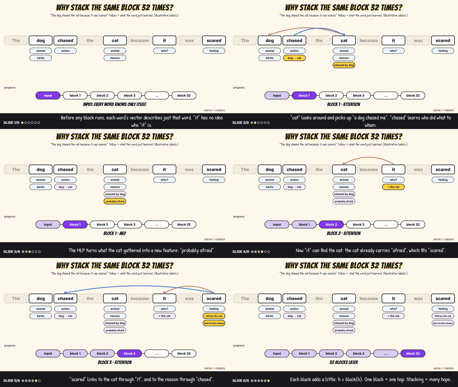
Each block doesn’t replace a word’s vector; it adds a small correction to it:
This is called a residual connection. It’s like editing a draft several times: each pass improves the text a little instead of rewriting it from scratch. Notice the shape: the original plus a small learned addition. Keep it in mind, because LoRA’s formula has exactly the same shape.
Why 32, and not 3 or 1,000? It’s a design trade-off, not a law. More blocks give more hops and more capacity, and bigger models generally do better when there’s enough data and compute to train them. But every block costs memory and time for every word, and the gains shrink after a point. Designers balance depth (the number of blocks) against width (how many numbers describe each word): Llama 2 7B uses 32 blocks of width 4,096, while Llama 2 70B uses 80 blocks of width 8,192.
Repeating one design also keeps things simple: to build a bigger model, you mostly add blocks. And it makes LoRA easy to apply, because the same 7 kinds of matrices appear in every block, so one setting can cover them all.
What fine-tuning actually changes: learning ΔW
The apartment example
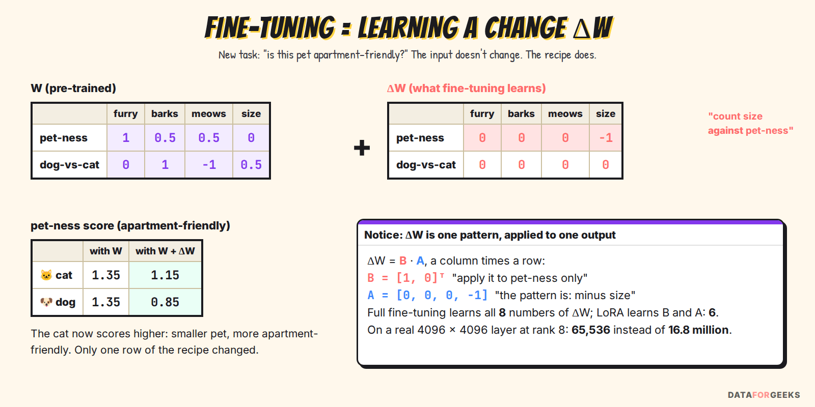
Back to our pet recipe W. Now give the model a new task: “Is this pet apartment-friendly?” Small pets should score higher. The inputs don’t change; a cat is still a cat. What must change is the recipe: the pet-ness row should count size against the animal. So fine-tuning learns a change to the weights:
Here, ΔW is all zeros except one cell: −1 in the pet-ness row, size column. The new pet-ness scores are cat 1.35 − 0.2 = 1.15 and dog 1.35 − 0.5 = 0.85. The cat now scores as more apartment-friendly, exactly what we wanted.
Why full fine-tuning is expensive
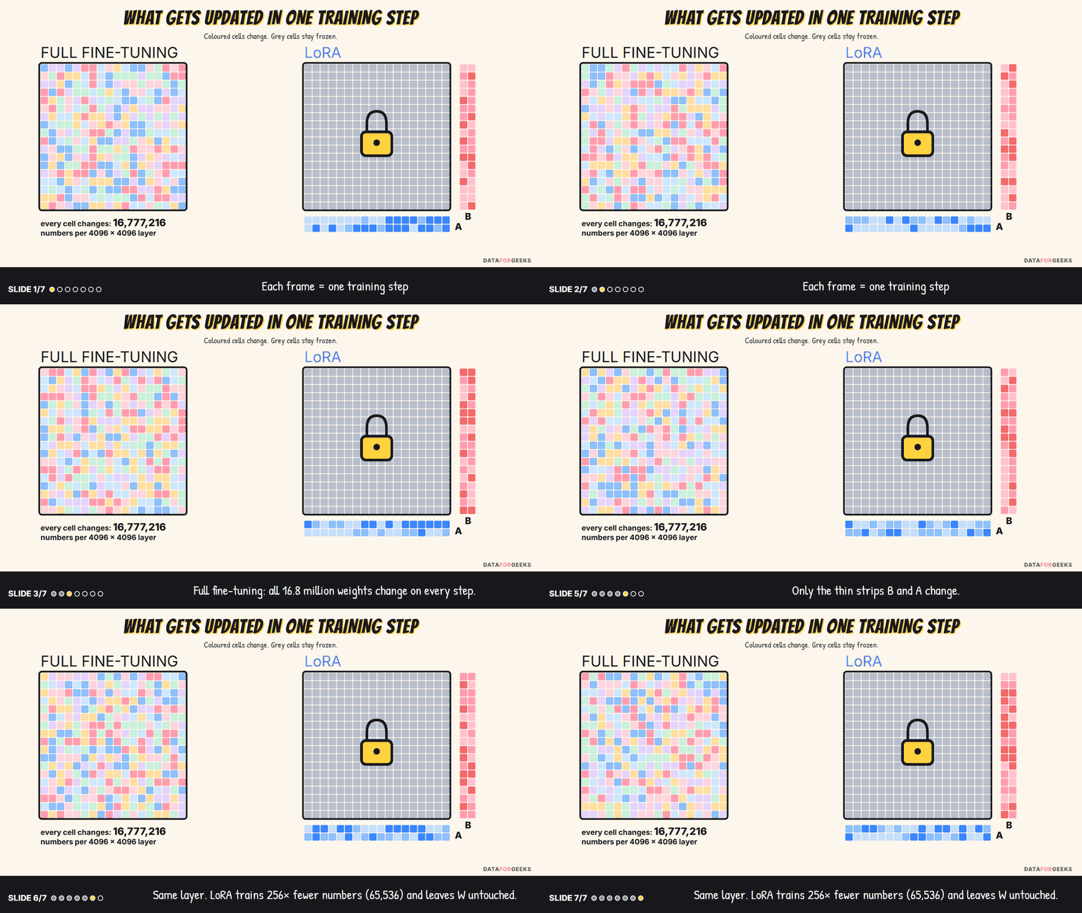
Full fine-tuning learns every number in ΔW, for every layer. That’s 8 numbers in our toy, but 16.8 million per real matrix. Each trainable number also needs a gradient, and the Adam optimizer keeps two more running averages per number (plus often a 32-bit master copy). That’s roughly 16 bytes per trainable parameter, before activations. For all 6.74 billion parameters, that’s about 108 GB.
But look closely at our ΔW. It’s really one idea (“subtract size”) applied to one output (pet-ness). LoRA fine-tuning starts from one question: does ΔW really need all those numbers, or is it usually made of a few simple patterns like this one?
What “low-rank” means in low-rank adaptation
The rank of a matrix is the number of different ideas (patterns) it’s made of. A low-rank matrix is built from only a few ideas, so it can be stored with far fewer numbers.
We already met a rank-1 change: the apartment ΔW. It had one idea, “minus size”, applied to one output, pet-ness. To see what rank really means, let’s make the example a little bigger.
One idea: a rank-1 change
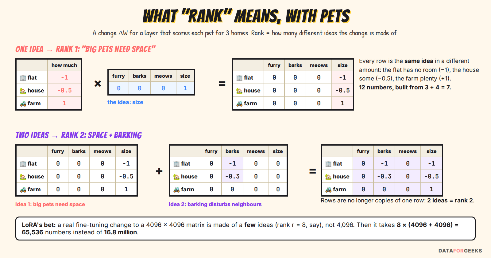
Imagine a layer with three outputs: how good a pet is for a 🏢 flat, a 🏡 house and a 🚜 farm. It reads the same four features as before (furry, barks, meows, size). So its weight matrix, and any change ΔW to it, has 3 rows (homes) × 4 columns (features) = 12 numbers.
Now fine-tune it with one new lesson: “big pets need space”. The flat has no room for a big pet (a lot less suitable), the house has some room (a little less), and the farm has plenty (more suitable). The change looks like this:
| ΔW | furry | barks | meows | size |
|---|---|---|---|---|
| 🏢 flat | 0 | 0 | 0 | −1 |
| 🏡 house | 0 | 0 | 0 | −0.5 |
| 🚜 farm | 0 | 0 | 0 | +1 |
Look at the rows. They’re all the same idea, “size”, just in different amounts: −1, −0.5 and +1. So we don’t need to store 12 numbers. We can store just two small lists and rebuild the table by multiplying them:
- The idea, a row: v = [0, 0, 0, 1], meaning “size, and nothing else”.
- How much each home uses it, a column: u = [−1, −0.5, +1].
Multiply every number in u by every number in v and you get the table back. For example, house × size = −0.5 × 1 = −0.5, and flat × furry = −1 × 0 = 0. That’s 3 + 4 = 7 numbers instead of 12. A matrix you can build from one column times one row is called rank 1 (mathematicians also call u × v an “outer product”).
A quick test for rank 1: can every row be written as one row times a number? Here, the flat row is −1 × the idea, the house row −0.5 ×, and the farm row +1 ×. Yes, so it’s rank 1.
Two ideas: a rank-2 change
Now teach a second, unrelated lesson at the same time: “barking disturbs neighbours”. The flat wants a quiet pet (−1 × barks), the house minds a little (−0.3 × barks), the farm doesn’t care (0). The total change is the two ideas added together:
| ΔW | furry | barks | meows | size |
|---|---|---|---|---|
| 🏢 flat | 0 | −1 | 0 | −1 |
| 🏡 house | 0 | −0.3 | 0 | −0.5 |
| 🚜 farm | 0 | 0 | 0 | +1 |
Try the test again. The farm row is [0, 0, 0, 1], but the flat row [0, −1, 0, −1] isn’t a multiple of it: it has a “barks” part the farm row doesn’t have. No single idea explains all the rows any more. You need two column-times-row pieces, one for size and one for barking, so this change is rank 2.
Why rank matters for LoRA fine-tuning
Each extra idea costs one more column-and-row pair. For our tiny 3 × 4 table, two ideas already cost 2 × (3 + 4) = 14 numbers, more than the 12 in the table, so there’s no saving at this size. The saving appears when the matrix is big and the number of ideas is small:
- A 4096 × 4096 change holds 16,777,216 numbers.
- If it’s made of just 8 ideas (rank 8), it can be built from 8 × (4096 + 4096) = 65,536 numbers: 256 times fewer.
That is the bet behind low-rank adaptation: when you fine-tune a model for a new task, the change to each weight matrix is made of a few ideas (“be more formal”, “spot this kind of attack”, “prefer this answer format”), not thousands. If that’s true, we can learn the few ideas directly and skip the rest. Choosing the LoRA rank r later simply means choosing how many ideas each adapter is allowed to learn.
Real changes are rarely exactly rank 8. They usually have a few strong ideas plus many tiny leftovers. So we need a way to find the strong ideas in any matrix and measure how strong each one is.
Finding the ideas: the SVD
For any matrix, there’s a standard tool that finds its ideas, strongest first: the singular value decomposition (SVD). It writes the matrix as a sum of rank-1 pieces:
Each term is one idea, exactly like our pets: viᵀ is the idea (a row; the ᵀ means “turned on its side”), ui is how much each output uses it (a column), and σi (sigma, a “singular value”) is how strong idea i is. SVD always lists the ideas strongest first: σ1 ≥ σ2 ≥ …
SVD on the pets change
Let’s run it on our rank-2 flat/house/farm change. To make it realistic, I added small random “leftovers” (±0.03) to every cell, because a real fine-tuning change is never perfectly clean. Then one NumPy call, np.linalg.svd, splits it into ideas:
- Idea 1: σ1 = 1.70, 87% of the change.
- Idea 2: σ2 = 0.65, 13% of the change.
- Idea 3: σ3 = 0.03, about 0%. That’s just the leftovers.
(The share of each idea is σi² divided by the sum of all σ², often called its energy.) Two strong ideas and one tiny one: SVD has told us the change is effectively rank 2, even though the leftovers technically make it rank 3.
YOU MIGHT BE WONDERING
Why “effectively” rank 2, if it’s technically rank 3?
Strictly, rank counts every σ that isn’t exactly zero. The clean change has σ = 1.72, 0.62 and exactly 0, so it’s rank 2. The leftovers turn that last σ into 0.035: tiny, but not zero, so the matrix is technically rank 3 (random noise almost always pushes a matrix to its maximum rank).
But idea 3 carries only 0.04% of the change. It isn’t a lesson the fine-tuning learned; it’s just the leftovers, like dust on a camera lens in a photo of a cat. Effective rank counts only the ideas above the noise. In NumPy you set the threshold yourself: np.linalg.matrix_rank(R) gives 3, while np.linalg.matrix_rank(R, tol=0.1) gives 2.
Real fine-tuning changes work the same way at a bigger scale. A 4096 × 4096 change is technically rank 4,096, because thousands of tiny σ’s are never exactly zero. What matters for LoRA is how many σ’s are big.
Now rebuild the change from only the strongest ideas:
- Keep 1 idea: 36% error. The flat’s size weight comes out as −1.17 instead of −1, and the farm even picks up a barking weight (+0.44) it never had. One idea is not enough.
- Keep 2 ideas: 2% error. Every number is back within 0.03 of the change we started with. The third idea was only noise, and we can throw it away.
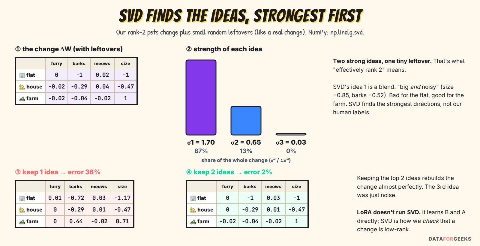
One surprise: SVD’s strongest idea isn’t exactly our “big pets need space”. It’s a blend, roughly “big and noisy” (size −0.85, barks −0.52), which is bad for the flat and good for the farm. The second idea covers what’s left. SVD finds the strongest directions in the numbers, not the labels a human would pick, but together the two ideas rebuild the same change. That’s also why, in the LoRA training animation, the learned B and A can look different from the “clean” answer while their product is right.
Effectively low-rank: the general rule
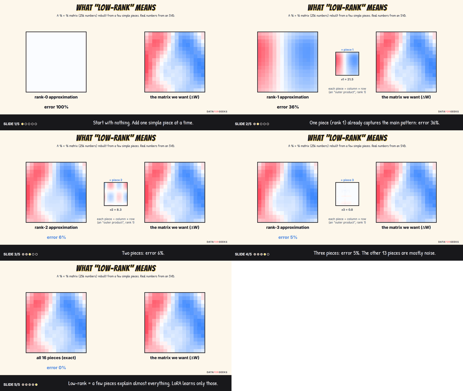
This is the general rule. If the first few σ’s are large and the rest are tiny, the matrix is effectively low-rank, and keeping only the top r ideas gives an almost perfect copy. (Keeping the top r ideas is in fact the best possible rank-r approximation, a result known as the Eckart–Young theorem.) The same thing works on a bigger matrix:
Is a real fine-tuning change low-rank?
Now the key observation behind LoRA. Earlier research found that fine-tuning large models works even when you restrict the update to a tiny random subspace (Aghajanyan et al., 2020, “intrinsic dimension”). Hu et al. took the next step and hypothesised that the weight change ΔW itself has a low “intrinsic rank”: a handful of ideas carry nearly all of it. If that’s true, we don’t need to learn 16.8 million free numbers per matrix. We only need to learn the few important ideas. That bet is what low-rank adaptation is named after.
One important note: LoRA doesn’t run SVD. Low-rank adaptation only borrows the idea. SVD is a tool to check whether a change is low-rank. LoRA skips the full change entirely and learns the few ideas (B and A) directly during training.
YOU MIGHT BE WONDERING
Is ΔW really low-rank, or is this just a nice story?
It’s an empirical observation, not a law. The LoRA paper showed that very small ranks (even r = 1 on GPT-3) matched full fine-tuning on their benchmarks, and that the top directions learned at different ranks overlap heavily. We’ll check it ourselves on a real model further down: the change made by full fine-tuning concentrates far more of its energy in its top few directions than a random matrix would. But it also has limits: tasks that need a lot of new knowledge push LoRA’s capacity, which we’ll cover in the limitations section.
How LoRA fine-tuning works
The LoRA trick: ΔW = B·A
LoRA fine-tuning (low-rank adaptation) freezes the pre-trained weight matrix W and learns its update as the product of two small matrices, ΔW = B·A, whose inner size r (the rank) is tiny. Instead of learning a full grid, it learns a “tall thin” matrix B and a “short wide” matrix A:
Multiply a (dout × r) matrix by an (r × din) matrix and you get a full (dout × din) matrix, the right shape to add to W. But because everything passes through only r numbers in the middle, BA can have rank at most r. That’s the low-rank bet, built into the shapes. The symbol ≪ means “much smaller than”: r is 8 or 16 when din and dout are 4096.
Remember the apartment example? Its ΔW is exactly B·A with LoRA rank r = 1: B = [1, 0]ᵀ (2 × 1, “apply it to pet-ness only”) and A = [0, 0, 0, −1] (1 × 4, “the pattern is minus size”). LoRA learns those 6 numbers instead of all 8. On a real 4096 × 4096 layer at r = 8, it’s 65,536 instead of 16.8 million: the same idea, at a scale where it matters.
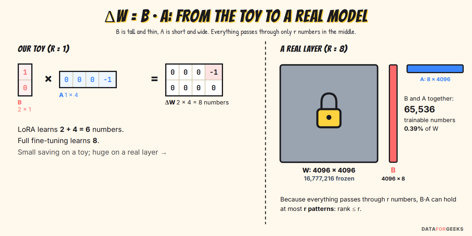
Think of B and A as a zip file for ΔW. A (r × din) compresses the input into r numbers: “how much of each pattern is in this input?” In the pets example, A asks one question: “how big is it?” B (dout × r) decompresses: “for each pattern, how should each output change?” In the pets example: “lower the pet-ness score by that much, leave dog-vs-cat alone”.
The forward pass: h = Wx + (α/r)·B(Ax)
With LoRA, each adapted layer computes:
Read it left to right:
- Wx: exactly what the original model computes. W is frozen; it never gets a gradient update.
- Ax: squeeze the input down to r numbers.
- B(Ax): expand those r numbers back up to dout.
- α / r: a fixed scaling factor. α (alpha) is a hyperparameter you choose; r is the rank. More on this below.
- +: add the small learned correction to the original output.
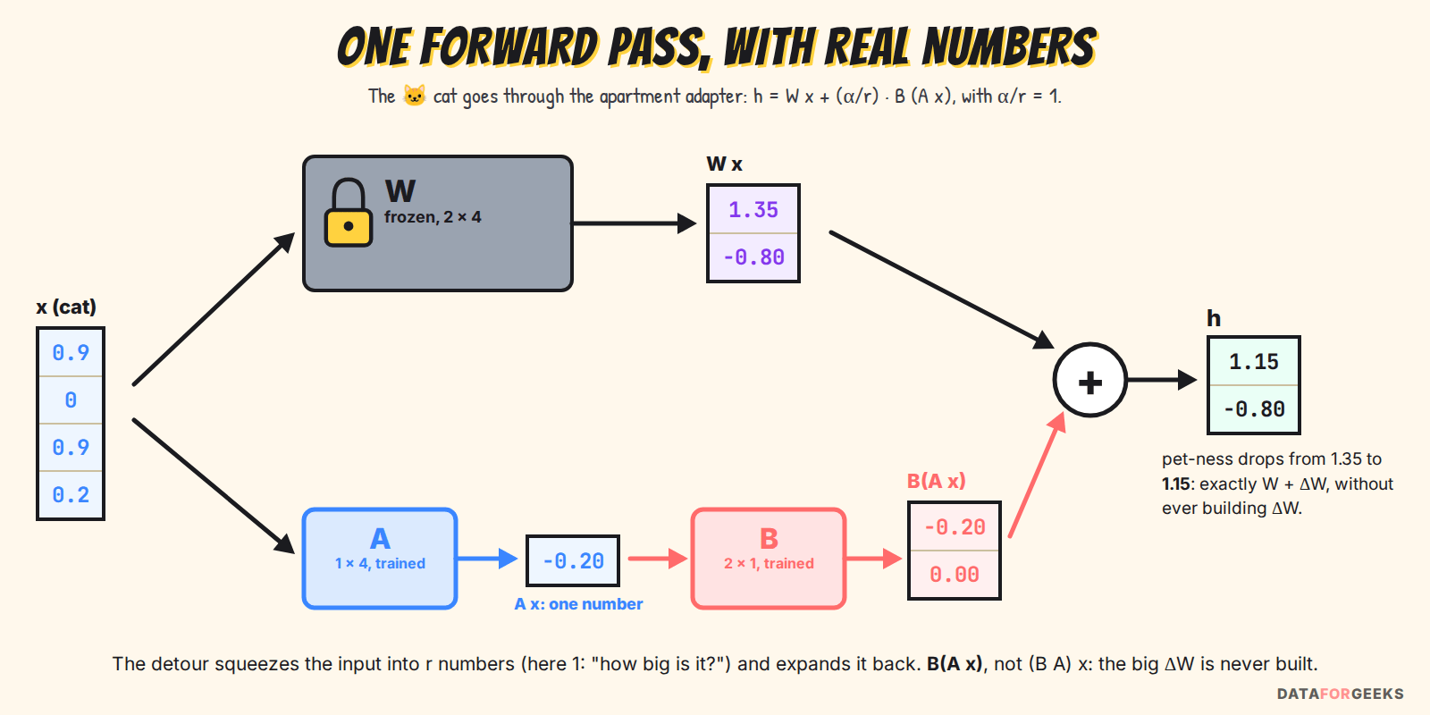
Let’s run it for the cat, with the apartment LoRA adapter and α/r = 1:
- Main road: W x = [1.35, −0.80], exactly the original output.
- Squeeze: A x = 0·0.9 + 0·0 + 0·0.9 + (−1)·0.2 = −0.2. One number: “minus how big it is”.
- Expand: B(A x) = [1, 0]ᵀ · (−0.2) = [−0.2, 0].
- Add: h = [1.35 − 0.2, −0.80 + 0] = [1.15, −0.80].
That’s exactly what W + ΔW gave earlier, but we never built ΔW. We only did two tiny multiplications on the side. Notice it’s the same shape as the residual connection between blocks: the original, plus a small learned addition.
In a real model, the same thing happens with thousands of numbers instead of four, and r patterns instead of one:
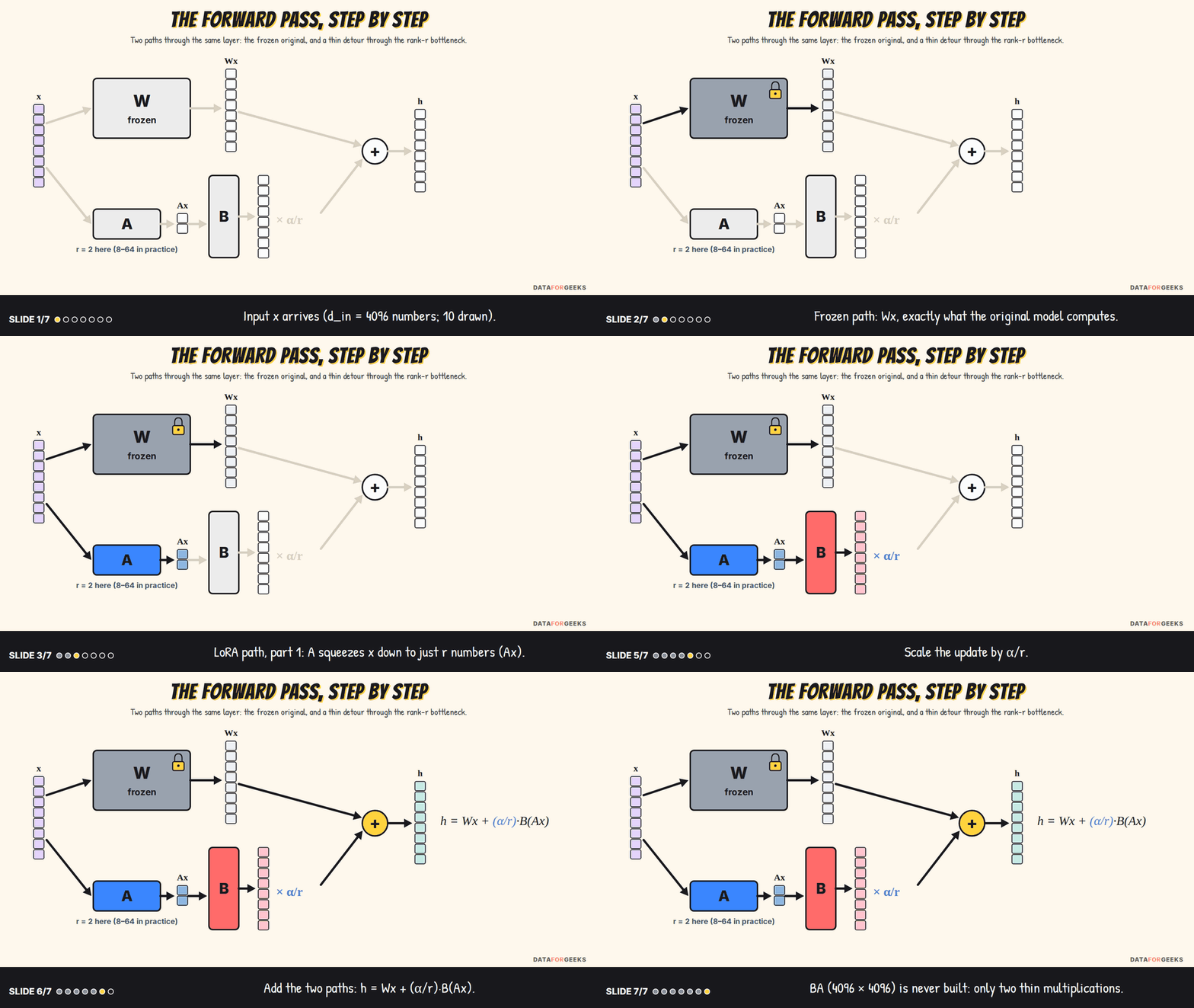
Notice the brackets: B(Ax), not (BA)x. Computing Ax first costs r·din multiplications, then B(·) costs dout·r. The dout × din matrix BA is never built during training. Per token, the extra work is tiny next to the frozen layer:
For 4096 × 4096 with r = 8: about 131K extra operations versus 33.5M. Under 0.4%.
LoRA rank and alpha: the scaling factor α/r
The LoRA rank r sets how much the adapter can learn, and the factor α/r keeps the update’s size roughly steady as r changes, so you don’t have to re-tune the learning rate every time you try a new LoRA rank. In the paper’s words, tuning α with Adam is “roughly the same as tuning the learning rate”, so the authors simply set α to the first r they tried and left it alone.
Think of α/r as a volume knob on the detour. In the pets example, the detour adds −0.2 to the cat’s pet-ness. With α/r = 0.5 it would add −0.1; with α/r = 2, −0.4. The knob doesn’t change what the LoRA adapter learned, only how loudly it speaks.
Why divide by the LoRA rank r? BA is a sum of r rank-1 pieces. With more pieces, the raw sum tends to get bigger, so dividing by r keeps its overall size steady. A common habit today is α = 2r, which makes α/r = 2 for any LoRA rank.
But dividing by r can over-correct. Kalajdzievski (2023) showed that with α/r, higher ranks learn more slowly and don’t deliver the gains they should. The fix, rank-stabilized LoRA (rsLoRA), divides by the square root instead:
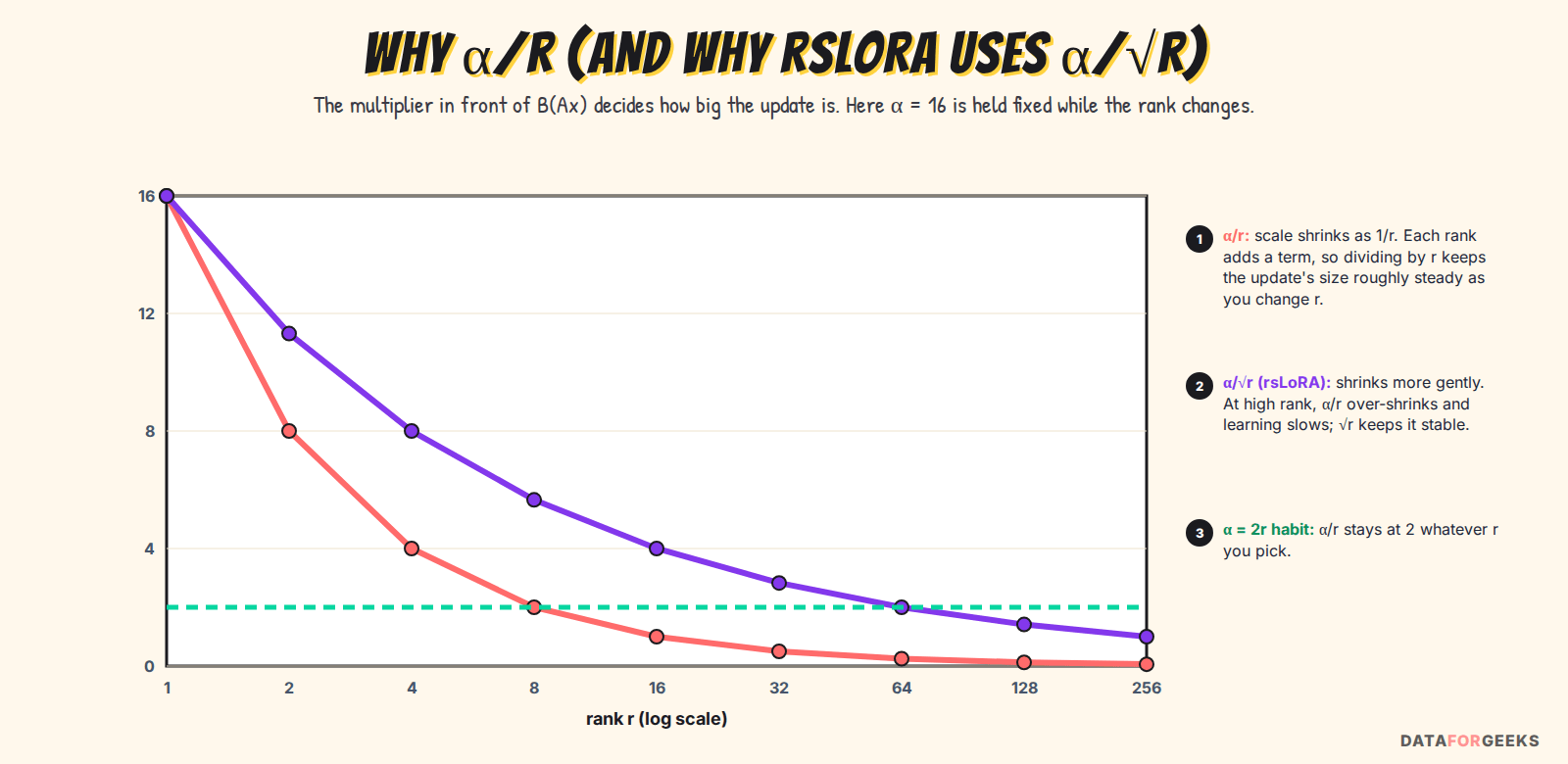
In Hugging Face PEFT this is one flag, use_rslora=True, which sets the scale to lora_alpha / math.sqrt(r). It matters most when you push the LoRA rank to 64, 128 or beyond.
Initialization: why B starts at zero
LoRA initializes A with small random values and B with zeros, so BA = 0 and the model at step 0 is exactly the original pre-trained model.
The original paper uses a random Gaussian for A. Hugging Face PEFT initializes A the same way PyTorch initializes a normal linear layer (Kaiming-uniform) and B with zeros. Either way, fine-tuning starts from a model that behaves exactly like the one you downloaded, so training can’t wreck it on step 0.
There’s a subtle consequence. Let g = ∂L/∂h be the gradient of the loss L with respect to the layer’s output (how much the loss would change if h changed). Using the chain rule on equation (6):
At step 0, B = 0, so ∂L/∂A = 0: A gets no gradient at all. B’s gradient isn’t zero, because it depends on Ax, and A is random. So on the very first step, only B moves. From step 1 on, B is non-zero and both matrices learn. (If both started at zero, neither would ever move. If both started random, the model would start out changed.) We verified this with a real 4096 × 4096 PyTorch layer too (code below): ‖∇A‖ = 0 and ‖∇B‖ > 0 at step 0.
Watching LoRA train on the pets example
Let’s watch LoRA fine-tuning happen on the pets example. I trained a rank-1 LoRA adapter on four animals (cat, dog, hamster, horse) with the apartment targets, starting from B = 0 and a small random A, using plain gradient descent (learning rate 0.5) on the squared error. W never changed:
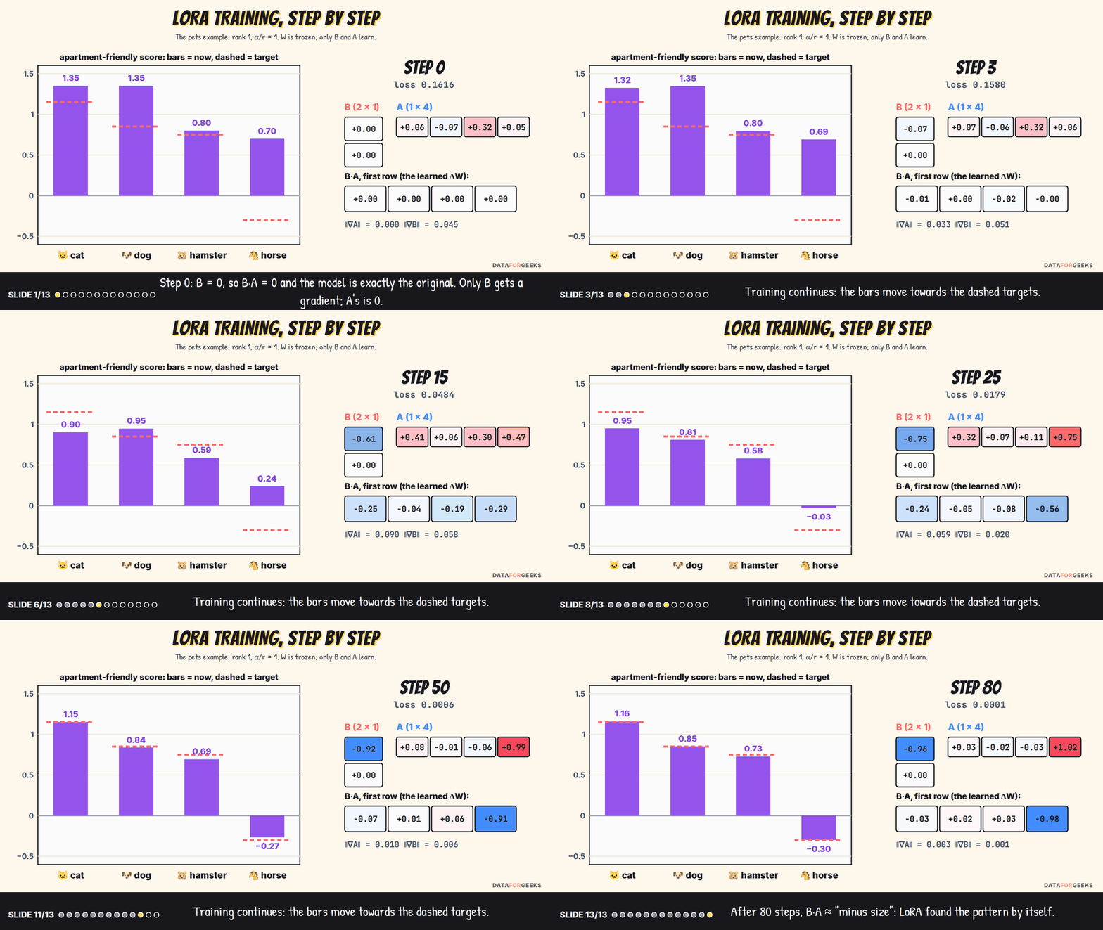
- Step 0: the scores are the original model’s, ‖∇A‖ = 0 and ‖∇B‖ = 0.045. Only B can move.
- Step 1: B is no longer zero, so A starts learning too (‖∇A‖ = 0.011).
- Step 80: the learned B·A is [−0.03, 0.02, 0.03, −0.98]: almost exactly “minus size”. Nobody told the adapter that pattern; it found it from four examples.
One detail worth noticing: the run ends with B ≈ −0.96 and A ≈ [0.03, −0.02, −0.03, 1.02], so the minus sign ended up in B instead of A. That’s fine. Only the product B·A matters, and many (B, A) pairs give the same product.
How many parameters LoRA saves
Full fine-tuning trains every entry of W. LoRA trains only B and A:
For a 4096 × 4096 projection with r = 8: 4096 × 4096 = 16,777,216 becomes 8 × (4096 + 4096) = 65,536, or 0.39%. Across a whole model:
| Setup (Llama-2-7B shapes) | Trainable parameters | % of 6.74B |
|---|---|---|
| Full fine-tuning | 6,738,415,616 | 100% |
| LoRA as in the paper: q, v only, r = 8 | 4,194,304 | 0.06% |
| LoRA today: all linear layers, r = 16 | 39,976,960 | 0.59% |
| LoRA, all linear layers, r = 64 | 159,907,840 | 2.37% |
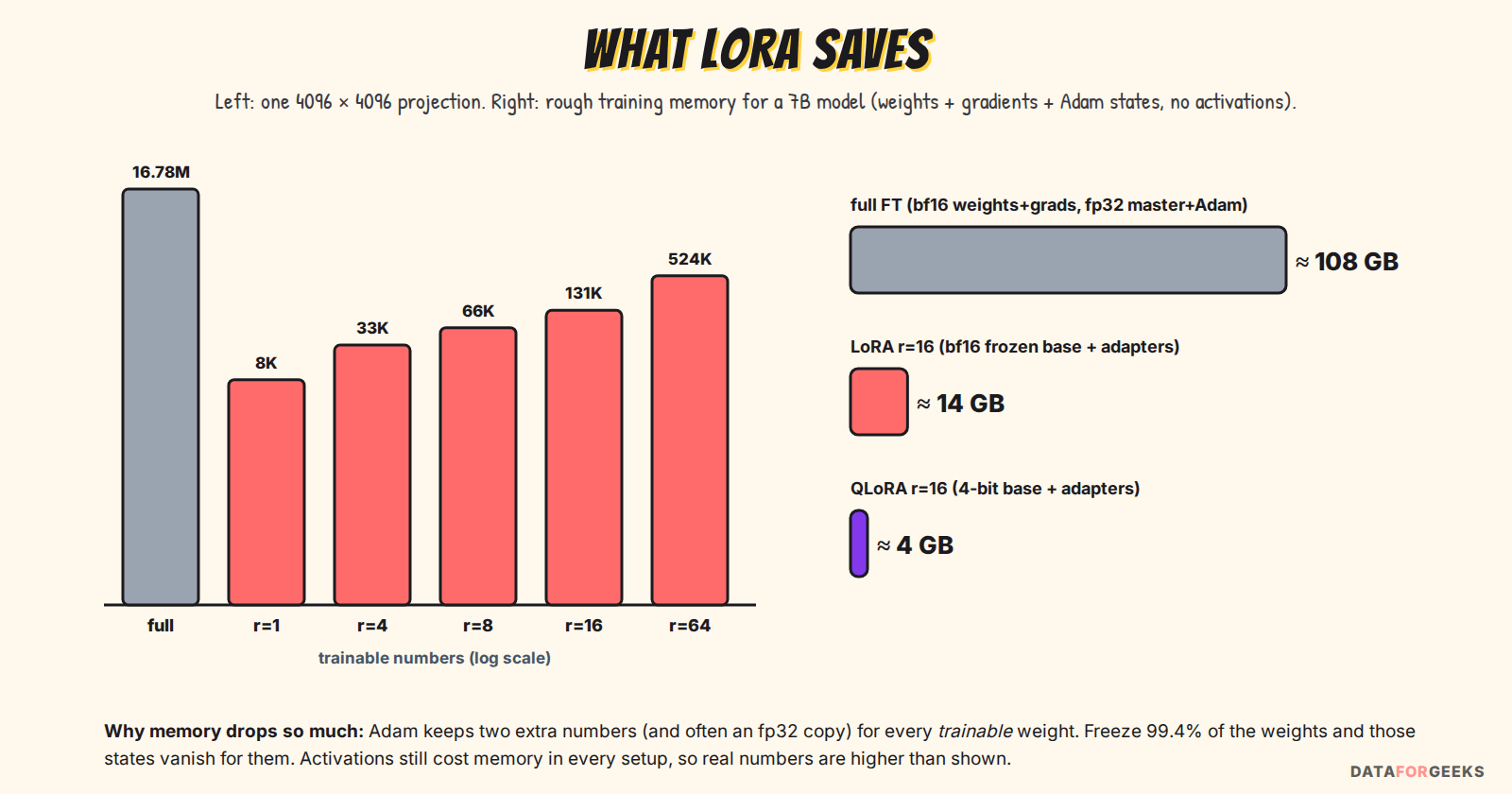
The memory story is bigger than the parameter count suggests. A rough rule for training memory, before activations:
For 7B: full fine-tuning ≈ 16 × 6.74B ≈ 108 GB; LoRA at r = 16 ≈ 2 × 6.74B + 16 × 40M ≈ 14 GB; QLoRA (4-bit base) ≈ 4 GB. Activations add more in every case, so real numbers are higher, but the gap is what matters: LoRA fine-tuning moves a 7B model from a multi-GPU server to a single card. The LoRA adapter you save is tiny too: ~80 MB for 40M parameters in bf16, instead of a 13.5 GB copy of the model.
Setting up LoRA fine-tuning in practice
Three choices matter most: which matrices get an adapter, how big the adapter is (its rank), and the learning rate.
Where to put LoRA in a transformer
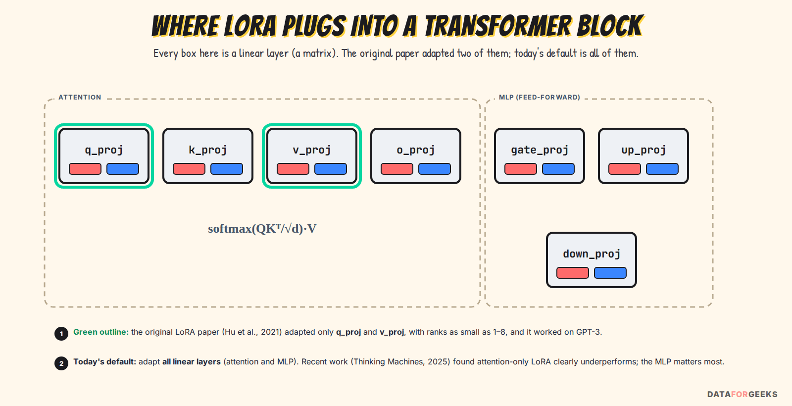
These are the 7 matrices of one block that we met with the pets: the four attention recipes and the three MLP recipes. Each box in that picture is a weight matrix W, just like our pet recipe but much bigger, and each gets its own LoRA adapter: a pair of small matrices, B (red) and A (blue).
The original paper applied LoRA only to the attention query and value projections (Wq, Wv) with small ranks (r = 1–8), mostly for simplicity, and it worked on GPT-3. Practice has moved on: the common default today is r = 16–64 on all linear layers. The “LoRA Without Regret” study (Thinking Machines, 2025) found that LoRA “performs better when applied to all weight matrices, especially MLP and MoE layers”, and that attention-only LoRA significantly underperforms MLP-only LoRA. In PEFT, target_modules="all-linear" does this for you (it skips the output head).
LoRA fine-tuning isn’t only for chat models. It works the same way on encoder models like BERT or DeBERTa, for example a prompt-injection classifier: you set task_type="SEQ_CLS" in PEFT, and the small classification head on top is usually trained in full (it’s new, so there’s nothing to freeze), while the encoder’s linear layers get LoRA adapters. That’s the setup I used for the prompt-injection model.
Which LoRA rank should you pick?
The rank r is how many ideas each adapter can learn. Start at r = 16. For style, format or classification tasks (like my DeBERTa prompt-injection model), r = 8–16 is usually plenty. For a new domain or lots of training data, try 32–64 and compare on a held-out set. If doubling r doesn’t improve your validation metric, keep the smaller LoRA adapter: it’s cheaper to train, store and serve. At high ranks, turn on rsLoRA.
LoRA fine-tuning hyperparameters: learning rate and batch size
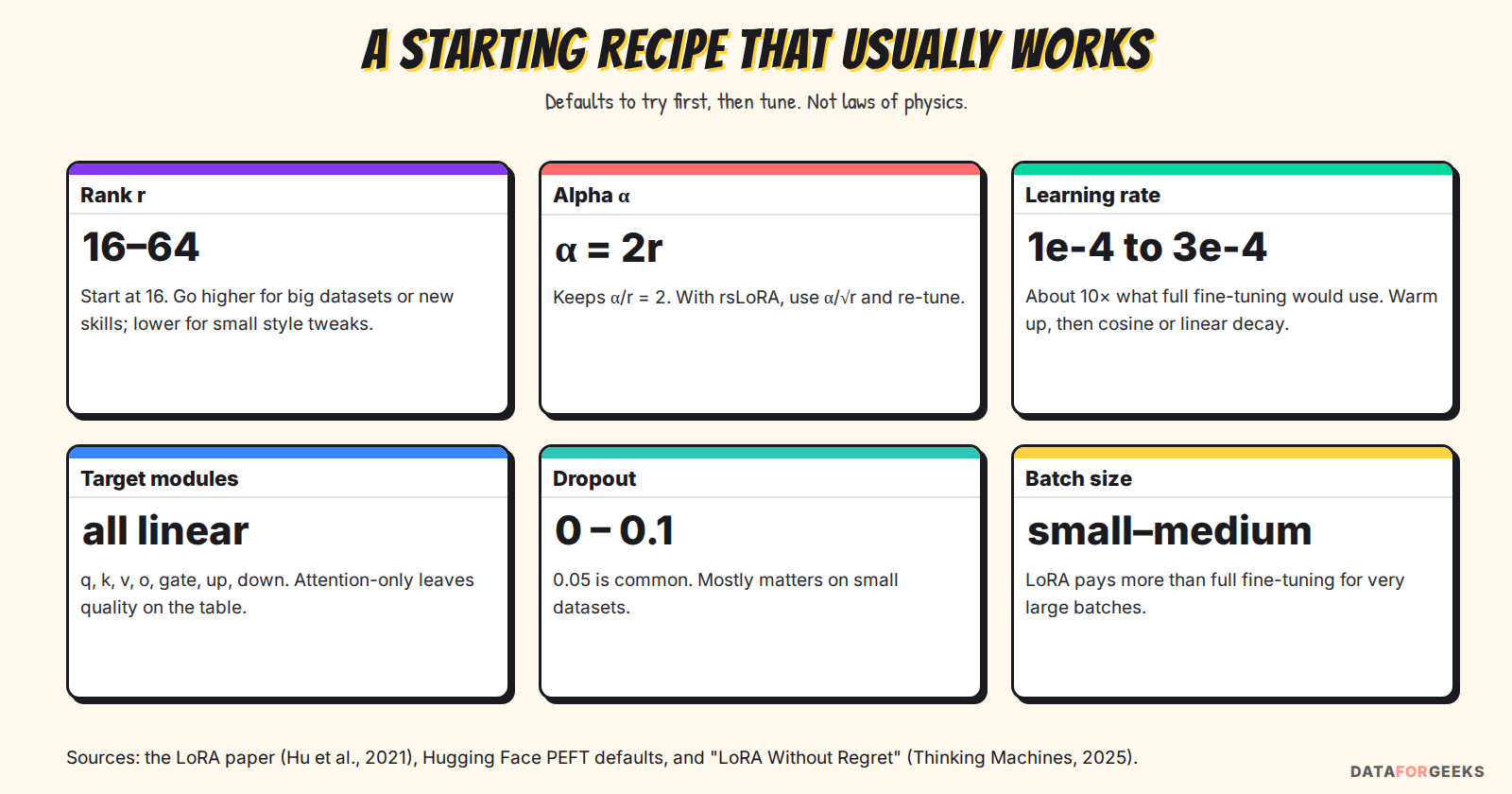
LoRA usually works best with a learning rate around 1e-4 to 3e-4, far higher than the 1e-5 to 5e-5 typical for full fine-tuning. The “LoRA Without Regret” experiments found the optimal LoRA learning rate was consistently about 10× the full fine-tuning one, and, thanks to the 1/r scaling, roughly independent of the rank. Intuitively: B starts at zero, every update is squeezed through r numbers and scaled by α/r, so each step moves the effective ΔW much less than a full-rank step would. A bigger step size compensates.
Two more practical findings from the same study: LoRA is less forgiving of very large batch sizes than full fine-tuning, and when a dataset is too big for the adapter’s capacity, LoRA falls behind. Both point to the same advice: start with the recipe above, then measure.
💡 Tip: Changing r? With α = 2r (or rsLoRA), you usually don’t need to re-tune the learning rate from scratch. Changing from full fine-tuning to LoRA? Multiply your learning rate by about 10 as a first guess.
LoRA fine-tuning vs full fine-tuning on a real model
Formulas are nice; numbers are better. Here’s LoRA fine-tuning measured against full fine-tuning. I fine-tuned a real (small) language model, DistilGPT-2 (82M parameters), on CPU, on a new kind of text: the docstrings of the Python standard library. It isn’t a benchmark of large models; it isolates the two claims we care about.
- Full fine-tuning: all parameters trainable, AdamW, 150 steps, best of three learning rates (2e-05, 5e-05, 0.0001).
- LoRA: r = 8, α = 16, all linear layers (c_attn, c_proj, c_fc), 589,824 trainable parameters (0.7% of the model), best of three learning rates (0.0002, 0.0005, 0.001).
- Measured: loss on 64 held-out blocks (lower is better), and the singular values of the change ΔW that full fine-tuning made to the weights.
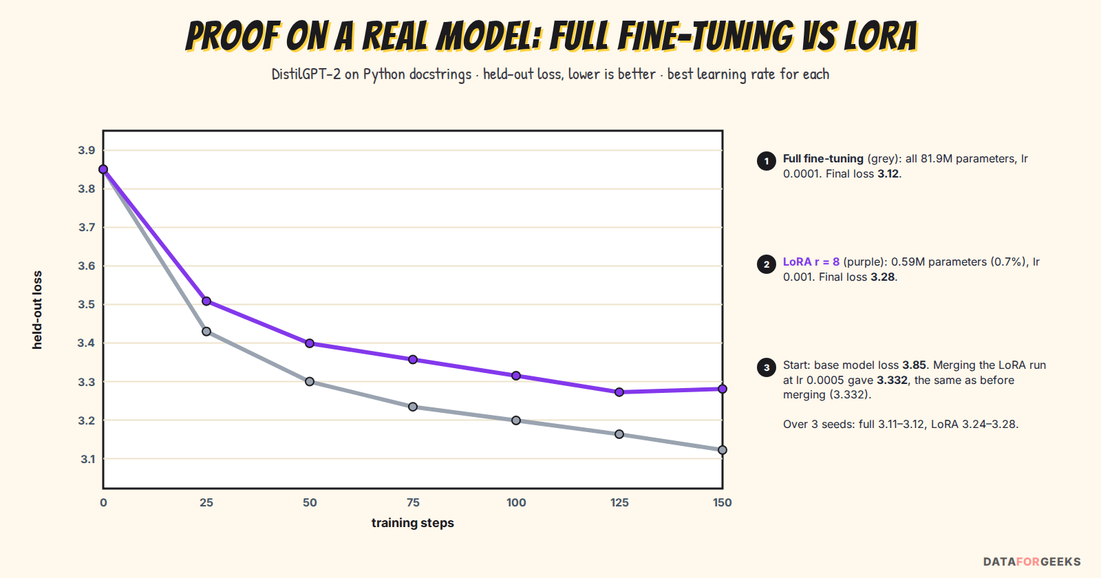
Both runs start from the same base loss, 3.85. After 150 steps, full fine-tuning reached 3.12 and LoRA 3.28, while training 0.7% of the parameters: LoRA recovered about 78% of the improvement that full fine-tuning made. Three details line up with the theory above:
- The learning rate. The best LoRA learning rate (1e-3) was 10× the best full fine-tuning one (1e-4), as “LoRA Without Regret” predicts. Both were at the top of the ranges I tried, so treat this as consistent with the rule, not proof of it. The usual 2e-4 recipe was the weakest LoRA run here (3.39); with only 150 steps, a bigger step size helped.
- The gap. At every 10× pair in the grid, LoRA trailed full fine-tuning by 0.11–0.16. On a small model with r = 8, there’s a real capacity cost.
- The merge. Merging the LoRA run at 5e-4 into the base weights gave a loss of 3.332, against 3.332 before merging: the same model, now with no extra layers.
What this is and isn’t: a small model, 150 steps on CPU, one dataset. I re-ran the best settings with 2 more random seeds (different batch order and LoRA initialization): full fine-tuning ended between 3.11 and 3.12, LoRA between 3.24 and 3.28, so the gap is stable, not noise. It checks the mechanics; it doesn’t say LoRA always trails full fine-tuning. Larger studies find LoRA often matches it when the dataset fits within the adapter’s capacity, which is exactly the limitation we’ll come back to.
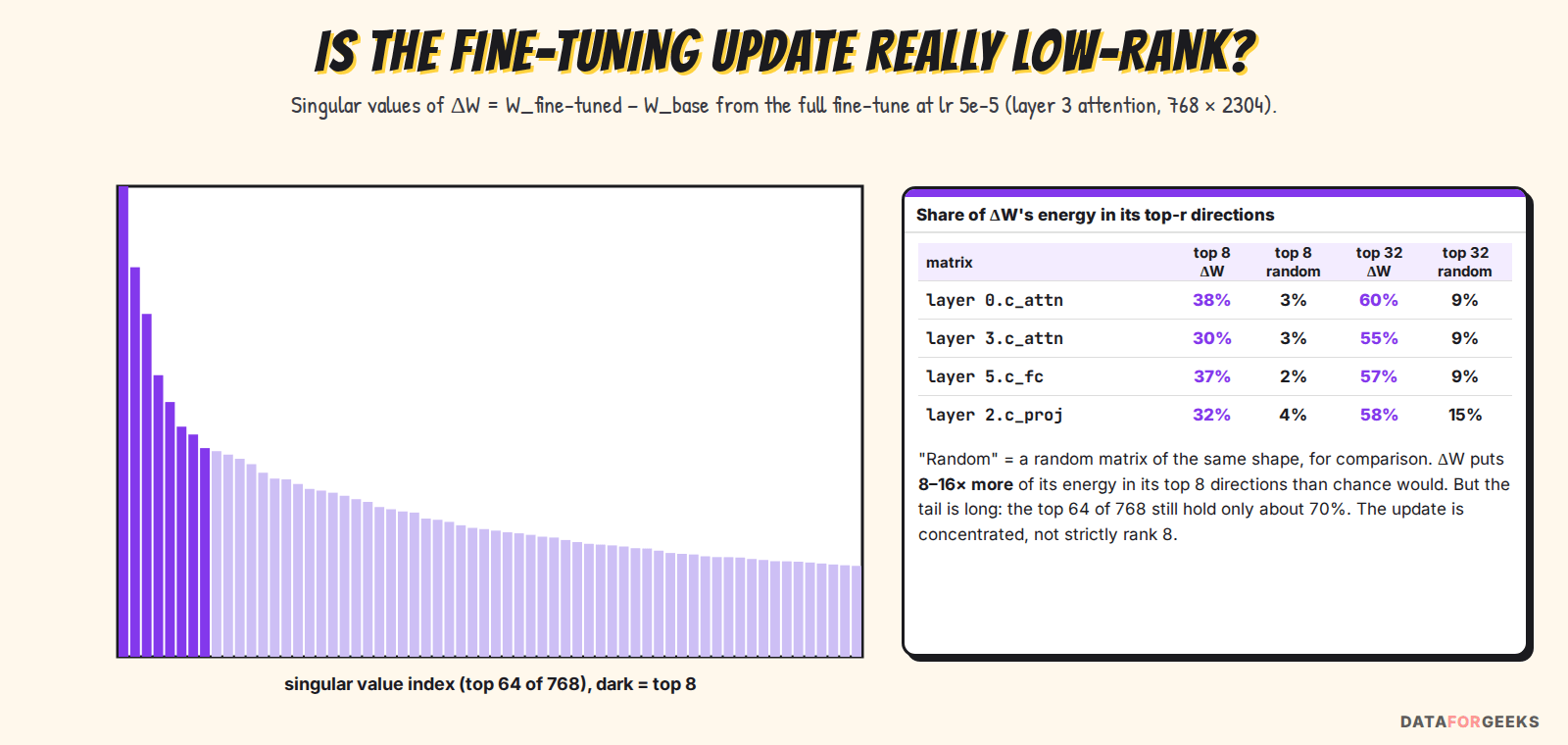
The second chart answers the question from the start of the post: is ΔW really low-rank? I took the change ΔW that full fine-tuning made to four weight matrices and computed its singular values. A matrix’s energy is the sum of its squared singular values, Σσi². In every matrix, the top 8 of 768 directions hold 30–38% of the energy, 8–16× more than in a random matrix of the same shape (2–4%). That’s the concentration LoRA bets on.
But it isn’t exactly rank 8: the top 64 directions hold only about 70%, and the rest is a long tail. So “low-rank” is an approximation that’s good enough to capture most of the change, not a law. That tail is one plausible reason the r = 8 adapter landed a little behind full fine-tuning here, and why raising r, or adapting all layers, helps on harder tasks.
🧩 My take: The part I find most useful isn’t the 0.4% of parameters. It’s that LoRA turns fine-tuning into something you can reason about: a frozen base, a small, separate, versionable file for each task, and a formula you can write on a whiteboard. That’s the kind of shape data engineers are good at operating, and it’s why I think LoRA fine-tuning belongs in every ML platform, next to the AI tools we already use day to day (I wrote about AI coding agents recently).
After training: merging and serving LoRA adapters
Once B and A are trained, you have two ways to use them: fold them into the model, or keep them separate and swap them per request.
Merging a LoRA adapter: zero extra latency
After training, a LoRA adapter can be merged into the base weights with one matrix addition per layer, producing a normal model with no extra inference cost.
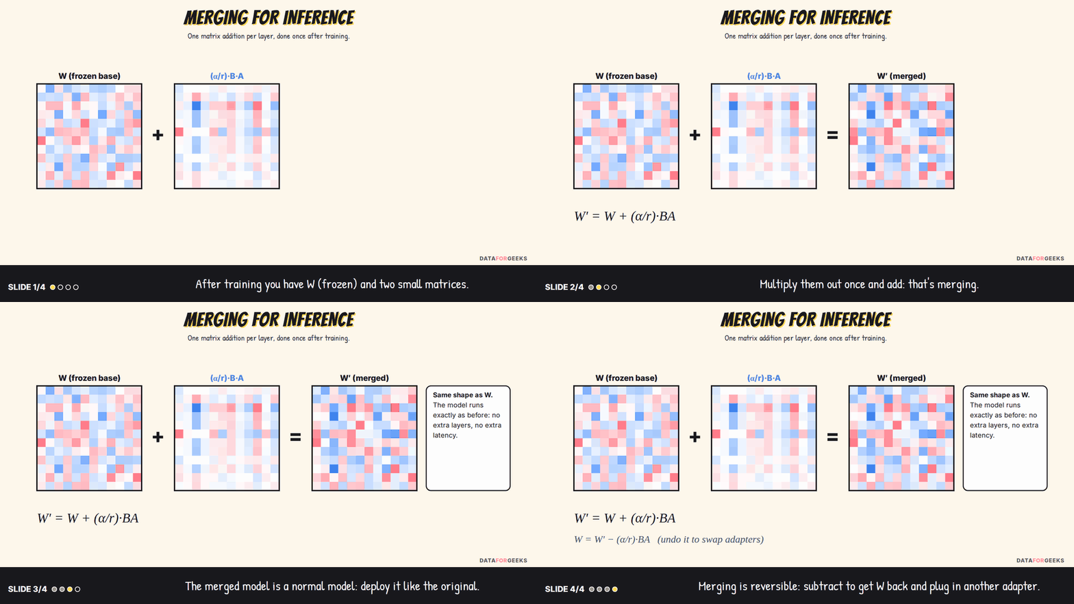
In the pets example, merging the apartment LoRA adapter gives a new pet-ness row [1, 0.5, 0.5, −1] (the size weight went from 0 to −1). The dog-vs-cat row doesn’t change. That single 2 × 4 table is the apartment model now: no detour, no extra step.
W′ has exactly the same shape as W, so the merged model runs at exactly the original speed: this is LoRA’s big advantage over older “adapter” methods that add extra layers. It’s also reversible: W = W′ − (α/r)·BA gets you back the base, so you can swap in a different adapter. In PEFT, merging a LoRA adapter is model.merge_and_unload(); our own check below shows the merged layer matches the unmerged one to within 1.2 × 10⁻⁶ (float32 rounding).
Merging a QLoRA adapter
QLoRA (Dettmers et al., 2023) stores the frozen base model in 4-bit NormalFloat (NF4) and trains 16-bit LoRA adapters on top, backpropagating through the quantized base. It made it possible to fine-tune a 65B model on a single 48 GB GPU. The forward pass becomes:
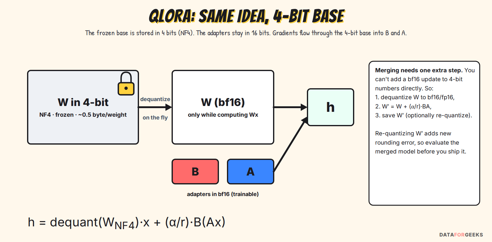
That creates a catch for QLoRA: you can’t add a 16-bit update to 4-bit numbers directly. To merge a QLoRA adapter, dequantize the base weights first (to fp16 or bf16), then compute W′ = W + (α/r)·BA and save the result. If you re-quantize W′ afterwards, you add a new round of rounding error on top of what the adapter learned, so evaluate the merged model before shipping it.
Serving many LoRA adapters without merging
Merging gives you one fine-tuned model. But a LoRA adapter is only tens of megabytes, while the base model is gigabytes. So there’s a second option: keep adapters separate and share one base model across many fine-tunes. For a batch of requests where request i uses adapter a(i):
The expensive part, Wxi, is shared by everyone in the batch; each request only adds its own tiny B·A detour. In the pets example, imagine three LoRA adapters on the same W: apartment (“minus size”), allergy-friendly (“minus furry”) and farm (“plus size”). Three different questions, three different answers, one shared model:
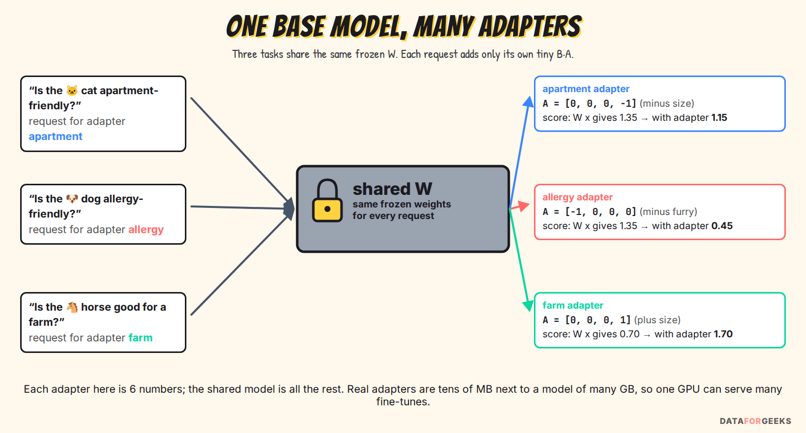
At real scale it looks like this:
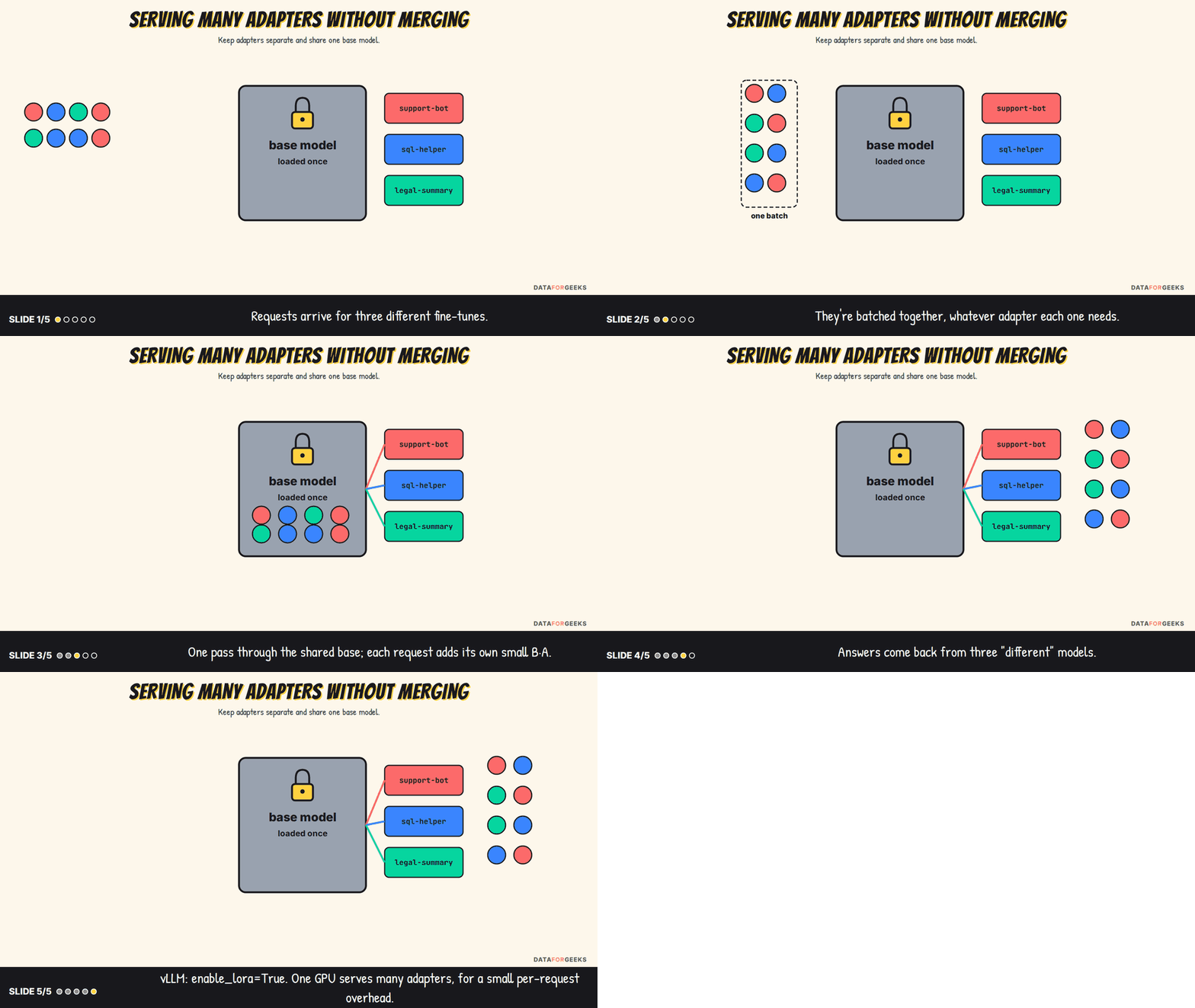
vLLM supports this with enable_lora=True (or --enable-lora on the server): requests for different adapters are processed together, in parallel with base-model requests, up to max_loras adapters at a time. You pay a small per-request overhead compared with a merged model, but one GPU can serve many fine-tuned variants: a support bot, a SQL helper and a summarizer, all from one copy of the weights.
| Merge the adapter | Serve adapters separately | |
|---|---|---|
| Latency | Same as the base model | Small extra cost per request |
| Models per GPU | One fine-tune | Many fine-tunes on one base |
| Swapping tasks | Re-merge (or keep several merged copies) | Pick an adapter per request |
| Best for | One high-traffic model | Many tenants, tasks or experiments |
LoRA fine-tuning in code
Note: the code in this post was written with the help of Claude (an AI assistant) to clarify the ideas. It’s illustration, not production code. Everything except the vLLM snippet was run while writing this post.
To run these, you only need Python with torch, transformers and peft installed. If your local Python setup is messy, my guide to a clean Python setup with pyenv gets you there in a few minutes.
Start with LoRA fine-tuning on the pets example. It runs in under a second with only NumPy, and it’s exactly what the training animation shows: forward pass (6), gradients (10), and only B and A being updated.
Next, LoRA from scratch in PyTorch: a frozen nn.Linear plus A and B, exactly equations (5), (6), (9) and (13).
Then the three checks from this post: identical output at step 0, zero gradient for A at step 0, and a merged layer that matches the unmerged one.
In real projects you’d use Hugging Face PEFT. This runs as-is on DistilGPT-2; swap the model name for Llama, Mistral or Qwen and it applies LoRA to every linear layer.
And serving several adapters with vLLM (from the vLLM docs; it needs a GPU, so I didn’t run it here):
Limitations of LoRA
- It learns less. “LoRA Learns Less and Forgets Less” (Biderman et al., 2024) found LoRA trails full fine-tuning on hard targets like code and maths when there’s a lot of training data, while forgetting less of what the base model knew. If your task needs lots of new knowledge, raise the rank or consider full fine-tuning.
- Capacity is capped by the LoRA rank. The update can never exceed rank r per matrix. For a style or format change, r = 8–16 is plenty; for a new domain with millions of examples, it may not be.
- Large batches hurt more than they do with full fine-tuning (Thinking Machines, 2025).
- Adapters are tied to their base model. An adapter trained on one checkpoint doesn’t reliably carry over to another, even a newer version of the same model; plan to retrain it when the base changes.
- Quantization adds error. With QLoRA, merging into a re-quantized base can shift behaviour; test the merged model.
- It doesn’t make inference cheaper. LoRA saves training memory and storage. A merged model costs exactly what the base costs to run.
The LoRA family
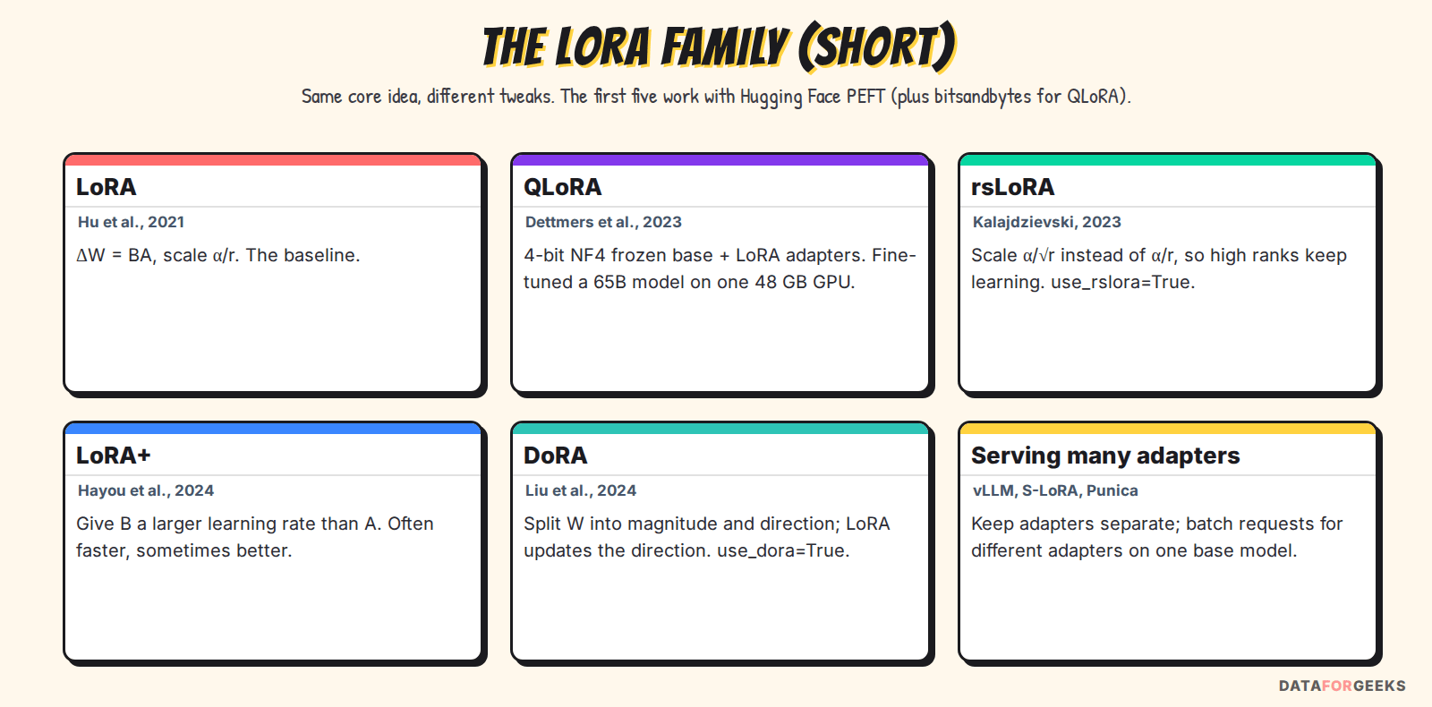
- QLoRA: 4-bit base, 16-bit adapters; the memory saver when LoRA fine-tuning still doesn’t fit on your GPU.
- rsLoRA: α/√r scaling so high ranks keep learning (
use_rslora=True). - LoRA+: a larger learning rate for B than for A.
- DoRA: splits each weight into a magnitude and a direction and applies LoRA to the direction (
use_dora=True).
Summary: LoRA fine-tuning in one page
| Concept | Formula | In plain words | In the pets example |
|---|---|---|---|
| Layer | h = W x | A recipe: weighted sums of the inputs | furry, barks, meows, size → pet-ness, dog-vs-cat |
| Attention and MLP | Wq, Wk, Wv, Wo; gate, up, down | 7 recipes per block, 224 in Llama 2 7B | cat → dog score 0.81, 69% attention |
| Fine-tuning | Wft = W + ΔW | Learn a change to the weights | “count size against pet-ness” |
| LoRA | ΔW = BA, r ≪ d | The change is low-rank: learn two thin matrices | B = [1, 0]ᵀ, A = [0, 0, 0, −1]: 6 numbers, not 8 |
| Forward pass | h = Wx + (α/r)·B(Ax) | Frozen path plus a thin, scaled detour | cat: 1.35 + (−0.2) = 1.15 |
| LoRA rank and scaling | α/r (rsLoRA: α/√r) | Rank = capacity; α/r = volume knob | r = 1, α/r = 1 |
| Initialization | A random, B = 0 | Starts exactly at the original model; only B moves on step 0 | step 0: ‖∇A‖ = 0, ‖∇B‖ = 0.045 |
| Parameters | r(din + dout) | 0.39% of a 4096 × 4096 layer at r = 8 | 1 × (4 + 2) = 6 |
| Merge | W′ = W + (α/r)·BA | Same shape, zero extra latency | pet-ness row becomes [1, 0.5, 0.5, −1] |
| Serve many | hi = Wxi + (α/r)·Ba(i)(Aa(i)xi) | One base, many adapters, one batch | apartment, allergy and farm adapters on one W |
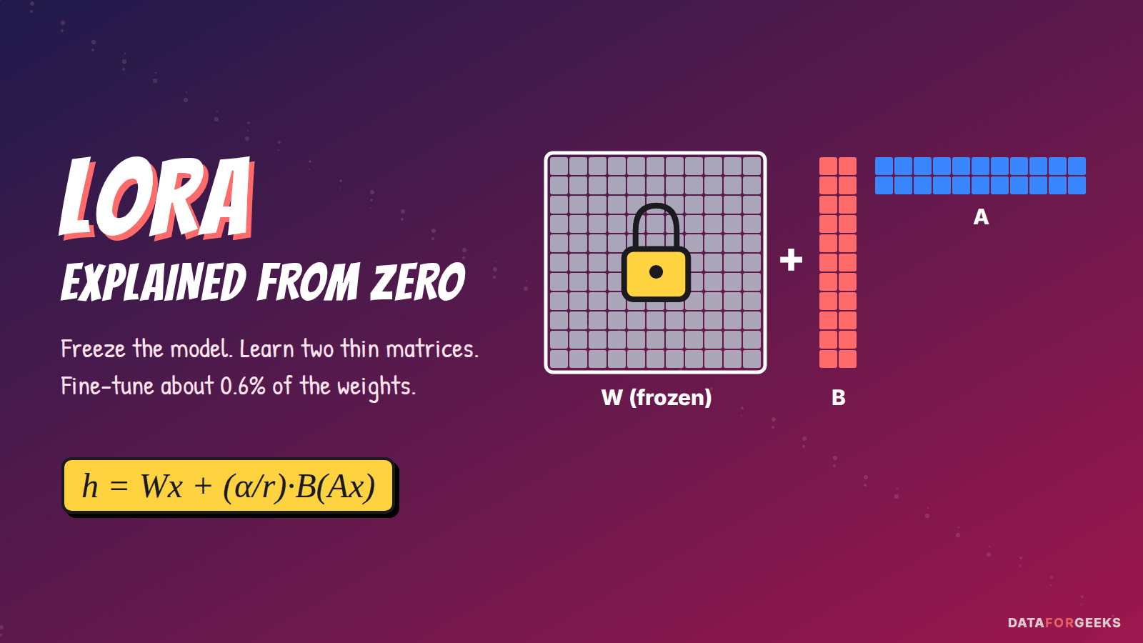
If you remember one line about LoRA fine-tuning, make it the one from the hero image: freeze the model, learn two thin matrices. Everything else, the scaling, the zero initialization, the merge, follows from that choice.
Have you fine-tuned with LoRA? Tell me in the comments which rank and learning rate worked for you, and on what kind of data. I’d love to compare notes.
Frequently asked questions
What is LoRA fine-tuning?
LoRA fine-tuning (Low-Rank Adaptation) is a way to fine-tune a large model without updating its weights. It freezes each pre-trained weight matrix W and learns the update as the product of two small matrices, B and A, so the layer computes h = Wx + (alpha/r) * B(Ax). Only A and B, the LoRA adapter, are trained, which is usually well under 1% of the model’s parameters.
What does h = Wx mean in a neural network?
It describes one linear layer. x is the input vector (for example, 4 numbers describing a cat: furry, barks, meows, size), W is the layer’s grid of learned weights, and h is the output vector. Each output number is a weighted sum of the inputs, using one row of W as the recipe. Fine-tuning changes W to W + ΔW; LoRA learns that change ΔW cheaply as B·A.
How does LoRA reduce the number of trainable parameters?
A full d_out x d_in weight matrix has d_out * d_in numbers. LoRA trains B (d_out x r) and A (r x d_in) instead, which is r * (d_in + d_out) numbers. For a 4096 x 4096 layer with r = 8, that is 65,536 instead of 16,777,216, about 0.39%.
What do rank r and alpha mean in LoRA?
The rank r is the inner size of the two LoRA matrices: the maximum rank of the learned update, and the main capacity knob. Alpha is a scaling hyperparameter: the update is multiplied by alpha/r (or alpha/sqrt(r) with rsLoRA). A common default is r = 16 to 64 with alpha = 2r, which keeps alpha/r at 2.
What LoRA rank should I use?
Start with r = 16 and alpha = 32. For style, format or classification tasks, a LoRA rank of 8 to 16 is usually enough. For a new domain or a large dataset, try 32 to 64 and compare on a held-out set; if doubling the rank doesn’t improve validation results, keep the smaller adapter. With rsLoRA (use_rslora=True), higher ranks keep learning effectively.
Why is the B matrix initialized to zero in LoRA?
With B = 0, the product BA is zero, so at step 0 the adapted model behaves exactly like the original pre-trained model. A is initialized randomly so that B receives a non-zero gradient on the first step; A’s own gradient is zero on that first step because it passes through B.
What learning rate should I use for LoRA?
Usually around 1e-4 to 3e-4, which is roughly 10 times higher than a typical full fine-tuning learning rate. Thanks to the 1/r scaling, the best learning rate is roughly independent of the rank, so you rarely need to re-tune it when you change r.
Which layers should LoRA be applied to?
The original paper applied LoRA only to the attention query and value projections. Current practice is to apply it to all linear layers (q, k, v, o and the MLP’s gate, up and down projections), because attention-only LoRA clearly underperforms. In Hugging Face PEFT, use target_modules=”all-linear”.
Does LoRA slow down inference?
Not if you merge it. After training, the adapter is folded into the base weights with W’ = W + (alpha/r) * BA, which has the same shape as W, so the merged model runs at exactly the original speed. If you keep adapters separate to serve many of them, each request pays a small overhead.
What is the difference between LoRA and QLoRA?
QLoRA is LoRA on top of a base model stored in 4-bit NF4 precision, which cuts memory much further: it fine-tuned a 65B model on a single 48 GB GPU. The adapters are still 16-bit. To merge a QLoRA adapter, you must first dequantize the base weights, then add the update.
Can one GPU serve multiple LoRA adapters?
Yes. Because adapters are small and share the same base model, servers such as vLLM can batch requests for different adapters together. In vLLM you enable it with enable_lora=True (or –enable-lora) and choose the adapter per request.
Is LoRA as good as full fine-tuning?
Often close, especially for style, format and task adaptation, and when LoRA fine-tuning is applied to all layers with a well-tuned learning rate. With very large datasets or tasks that need a lot of new knowledge, such as code or maths, full fine-tuning can learn more, while LoRA tends to forget less of the base model’s abilities. In a small DistilGPT-2 test in this post, LoRA with 0.7% of the parameters recovered about 78% of full fine-tuning’s improvement in 150 steps.
