Your table can only be sorted one way. Your users filter it ten different ways. That tension has shaped data lake design for years: sort by date and customer lookups crawl; sort by customer and every dashboard scans the whole table. Most teams quietly live with it, or keep two copies of the same data.
Apache Iceberg is getting a better answer: the Iceberg Hilbert curve sort order. Its standard compaction procedure, rewrite_data_files, can arrange rows along a Hilbert curve, a space-filling curve that keeps rows close on several columns at once, and does it more cleanly than the Z-order option Iceberg already had. The change itself is one new word in your SQL (source). What it unlocks is much bigger.
This one is personal for me. I’ve been following Iceberg for a few years now, and in May 2025 I wrote that Iceberg isn’t just a table format, it’s a philosophy shift: open, engine-agnostic, and smart enough to skip data using its own metadata. Hilbert clustering is that last idea taken one step further, and it closes a gap I’d been quietly waiting on.
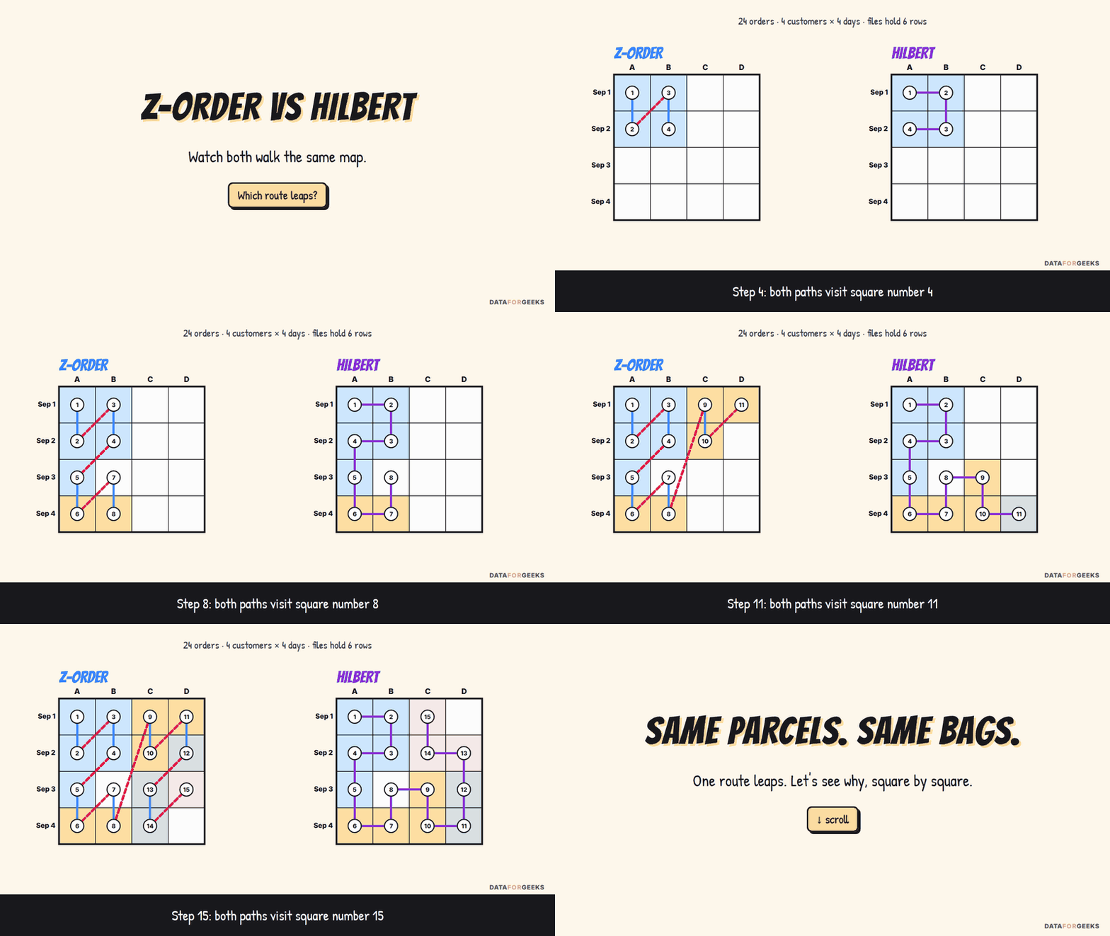
In this post I’ll explain the ideas from the ground up, and slowly. First, how queries skip files. Then a small table of 24 orders that we follow square by square, with Z-order and the Hilbert curve drawn side by side at every step, so you can see exactly where the two differ. Then the same idea at a million rows, with a simulation and real numbers, the limits nobody mentions, and finally what Hilbert clustering unlocks now that it’s coming to Iceberg and how to use it.
By the end you’ll be able to:
- explain Z-order vs Hilbert curve clustering to someone who has never heard of either, using one picture;
- work out by hand which file any row lands in, for both algorithms;
- explain why queries read fewer files, even though the query engine knows nothing about either curve;
- predict when clustering will disappoint you: skewed columns, too many columns, long strings, hot keys;
- decide between a plain sort,
zorderandhilbertfor your own Iceberg tables.
IN A HURRY? THE WHOLE STORY IN FIVE LINES
- The problem and the idea: queries are fast when each file covers a narrow range of values, but a table can only be sorted one way. Space-filling curves (Z-order, Hilbert) give rows one sort key that respects several columns at once.
- Z-order vs Hilbert curve: both picture rows on a map and number the squares along one path. Z-order’s path sometimes leaps across the map; Hilbert’s always steps to a touching square.
- Why it matters: a file that contains a leap gets a wide min/max range and is opened by more queries. In a million-row simulation, Hilbert opened 25–39% fewer files than Z-order on two-column filters.
- Why it’s exciting in Iceberg: cluster once and every engine that reads the table skips the same files, with no format switch. It unlocks one table for many query patterns, a real geospatial lakehouse and cheaper dashboards. Expected in Iceberg 1.12 with Spark 4.1.
- Limits: both curves struggle when one column’s values spread much wider than another’s, when you cluster on too many columns, and on single-column filters, where a plain sort still wins.
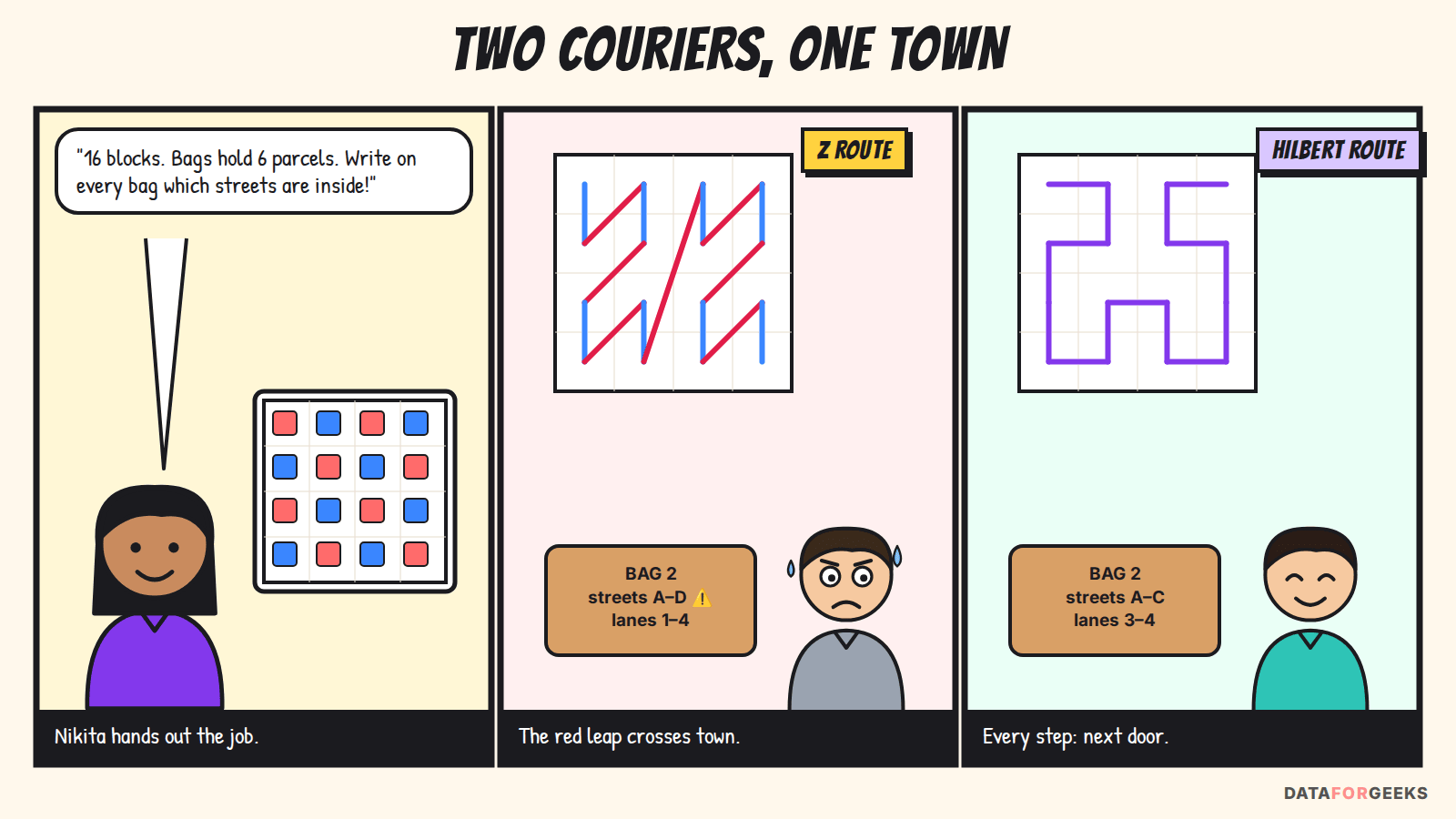
Keep that comic in mind. Parcels are rows, bags are files, and the note on each bag is the file’s label. Everything below is just this picture, done carefully.
Table of Contents
The problem: one table, many query patterns

Picture an events table with a few billion rows. The analytics team filters it by date for dashboards. The support team looks up one customer’s history. The product team asks for one region over a week. Same table, three access patterns, and each one wants the data arranged differently.
How a query skips files: min/max pruning (data skipping)

File pruning (also called data skipping) is how a query engine avoids opening data files that can’t contain matching rows, using per-file min/max statistics. A big Iceberg table is really thousands of Parquet files, and Iceberg’s metadata records the minimum and maximum value of each column in every file. When you run WHERE event_date BETWEEN '2026-09-10' AND '2026-09-12', the engine checks those ranges first and skips every file that can’t contain those dates, without opening it. This is file pruning, and it’s the single biggest lever for fast, cheap queries on large tables: fewer files opened means less I/O, less shuffle and a smaller compute bill.
I’ll call these per-file min/max values the file’s label: “customers A to B, dates Sep 1 to Sep 3”. The engine reads the labels first, skips every file whose label can’t match, and never opens those files. So the whole game is simple to state:
Narrow labels → more files skipped → faster, cheaper queries.
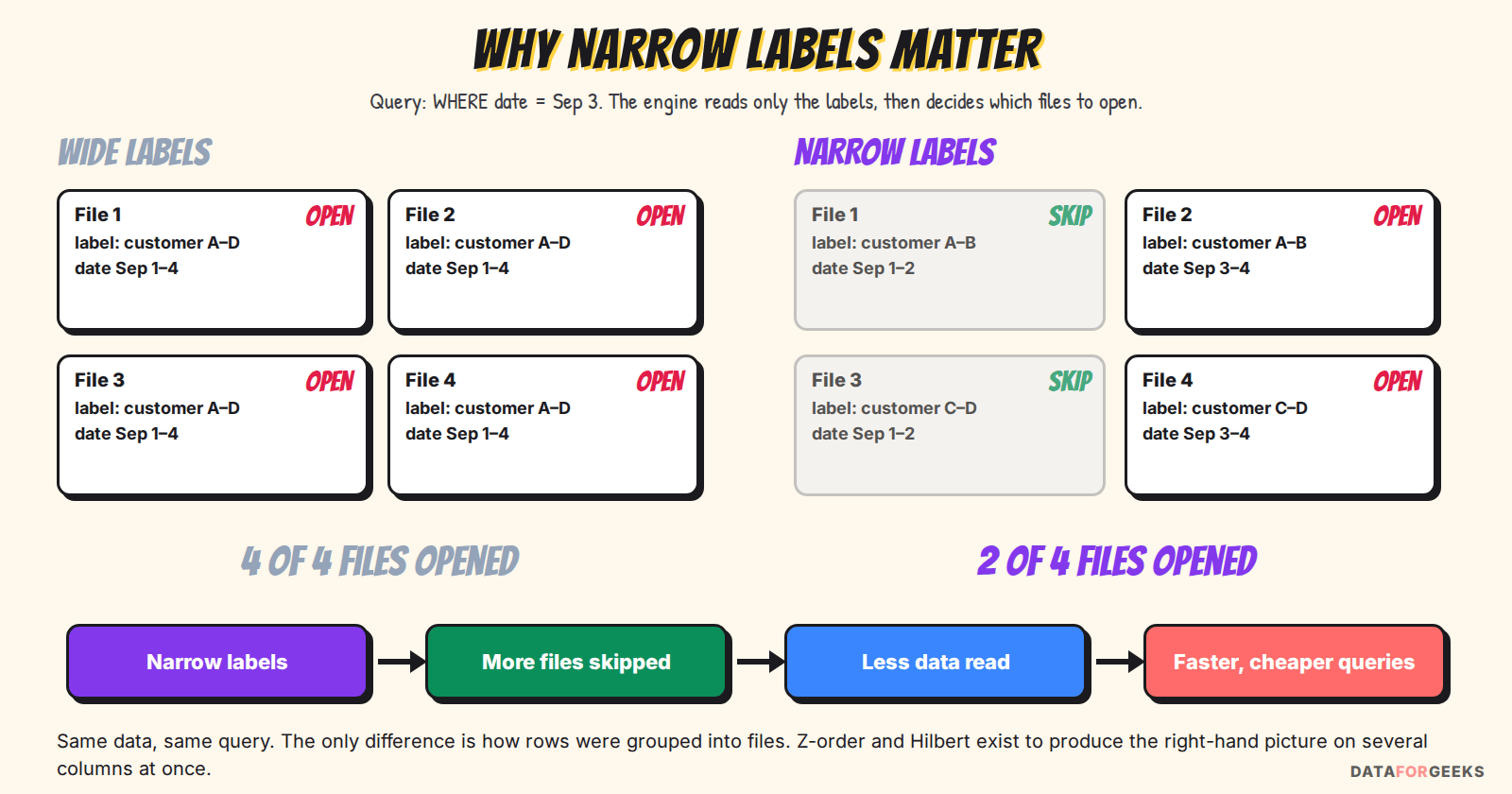
Pruning only works if file ranges are narrow. If every file holds rows from the whole month, every file’s range covers your three days, and nothing gets skipped. Two details are worth knowing. By default Iceberg keeps these ranges for the first 100 columns and truncates string ranges to 16 characters. And inside each Parquet file, row groups carry their own min/max too, so good clustering pays off twice.
Why one sort order isn’t enough
The classic fix is to sort. Sort by event_date and each file holds a thin slice of dates, so date filters prune beautifully. But the customer lookup and the region query now hit files that each contain every customer and every region. In the simulation later in this post, a table sorted by two columns had to open all 64 files for a filter on the second column alone.
Hence the old workaround: keep a second copy of the table sorted differently, and pay for the storage, the pipelines and the “which copy is right?” conversations. What we really want is a single arrangement that keeps files narrow on several columns at once. That’s what space-filling curves do.
Partitioning first, clustering second: where you name the columns
These two are often confused, so let’s separate them before we start:
| Partitioning | Clustering (Z-order or Hilbert) | |
|---|---|---|
| What it does | Splits the table into folders, e.g. one per month | Decides which rows share a file inside each folder |
| Where you name the columns | When you create the table | When you run the rewrite/compaction job, e.g. “cluster by customer and date” |
| When it happens | On every write | When the compaction job runs (typically on a schedule) |
| How queries use it | Skip whole folders | Skip files inside the folders that remain |
So yes, you name columns twice, for two different jobs. In our example, the table is partitioned by month, and we cluster the September folder by customer and date.
💡 Tip: Want to see pruning on your own tables? In the Spark UI, the SQL tab’s scan node for an Iceberg table reports scanned vs skipped data files, and the db.table.files metadata table shows each file’s lower and upper bounds (readable_metrics). My Spark UI debugging guide walks through the SQL tab in detail.
Z-order vs Hilbert curve, square by square: a worked example
Before we look at how Iceberg does this at scale, let’s slow all the way down. We’ll take one tiny table and follow every row through both algorithms, one step at a time. Keep the couriers from the comic in mind: rows are parcels, files are bags, and each bag’s note is the file’s label.
Our example: 24 orders, 4 customers, 4 days
September has 24 orders from four customers (A, B, C, D) over four days (Sep 1 to Sep 4). Files hold 6 rows each, so we’ll end up with 4 files.
Here is the complete dataset. Keep it handy: every picture below uses exactly these 24 rows, so if you get lost at any step, come back here and trace an order through.
| Order | Customer | Date | Amount | Order | Customer | Date | Amount |
|---|---|---|---|---|---|---|---|
| #1 | A | Sep 2 | ₹480 | #13 | D | Sep 2 | ₹340 |
| #2 | B | Sep 4 | ₹1500 | #14 | A | Sep 1 | ₹560 |
| #3 | D | Sep 4 | ₹1500 | #15 | D | Sep 2 | ₹700 |
| #4 | D | Sep 3 | ₹1200 | #16 | A | Sep 3 | ₹340 |
| #5 | C | Sep 2 | ₹120 | #17 | C | Sep 1 | ₹950 |
| #6 | D | Sep 3 | ₹1200 | #18 | B | Sep 4 | ₹250 |
| #7 | D | Sep 4 | ₹1200 | #19 | B | Sep 1 | ₹1200 |
| #8 | D | Sep 4 | ₹700 | #20 | A | Sep 1 | ₹560 |
| #9 | B | Sep 2 | ₹120 | #21 | C | Sep 4 | ₹950 |
| #10 | C | Sep 4 | ₹480 | #22 | C | Sep 3 | ₹1500 |
| #11 | D | Sep 3 | ₹120 | #23 | D | Sep 1 | ₹340 |
| #12 | A | Sep 4 | ₹950 | #24 | D | Sep 2 | ₹250 |
orders table for September, in the order the rows arrived (orders #1–#12 on the left, #13–#24 on the right).Here is what the files look like if we write rows in the order they arrived, with no clustering at all:
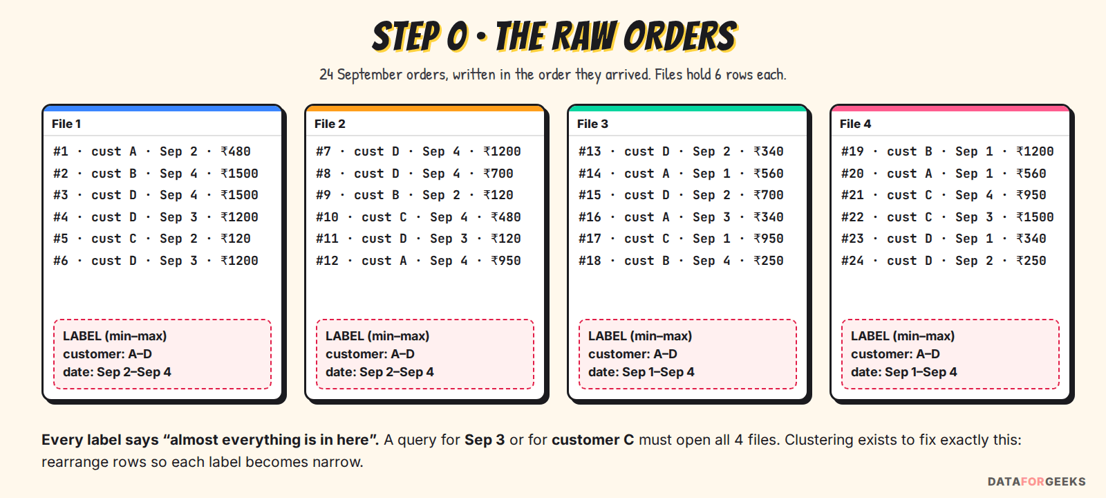
Every label says “almost everything is in here”. A query for Sep 3 opens all 4 files. So does a query for customer C. The statistics exist, but they’re useless. Let’s fix that, one step at a time.
Put every order on a map
Draw a grid: one column per customer, one row per day. Every order drops into the square for its customer and its day. Order #14 is customer A on Sep 1, so it goes in the top-left square. Order #22 is customer C on Sep 3, so it goes in the third column, third row.
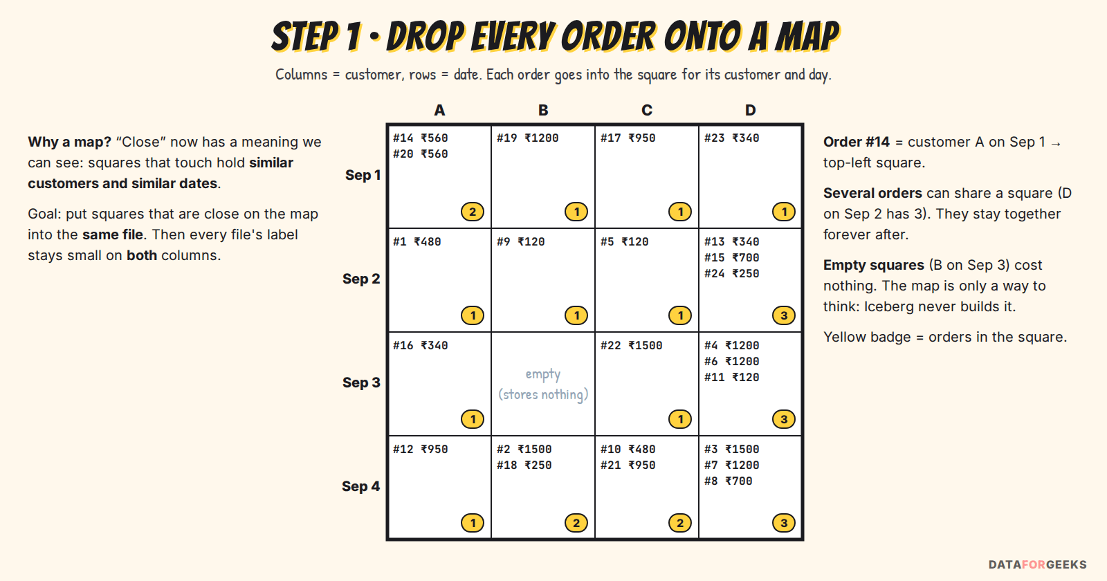
Three things to notice, because they’ll matter later:
- “Close” now means something you can see. Two squares that touch hold similar customers and similar dates. Our goal becomes: put squares that are close on the map into the same file.
- Squares can hold several rows. Customer D ordered three times on Sep 2. Rows in the same square always travel together.
- Empty squares cost nothing. Nobody ordered for customer B on Sep 3. Nothing is stored for it. In fact the map is never built at all; it’s only a way to think. The computer just works out a number for each row, as we’ll see.
YOU MIGHT BE WONDERING
With a million customers and five years of dates, isn’t this map enormous?
It would be, if anyone built it. Nobody does. Each row gets one small number (its position on the path we’re about to draw), rows are sorted by that number, and the number is thrown away. The work grows with the number of rows you have, never with the number of possible squares.
Split the map into quarters: where the two algorithms part ways
Both algorithms now do the same thing: draw one continuous path that visits every square exactly once. Squares next to each other on the path will end up in the same file. The path is drawn with one repeated trick:
Split the map into 4 quarters. Decide the order to visit the quarters. Then do the same thing inside each quarter.
Here is the top level, with Z-order on the left and the Hilbert curve on the right:
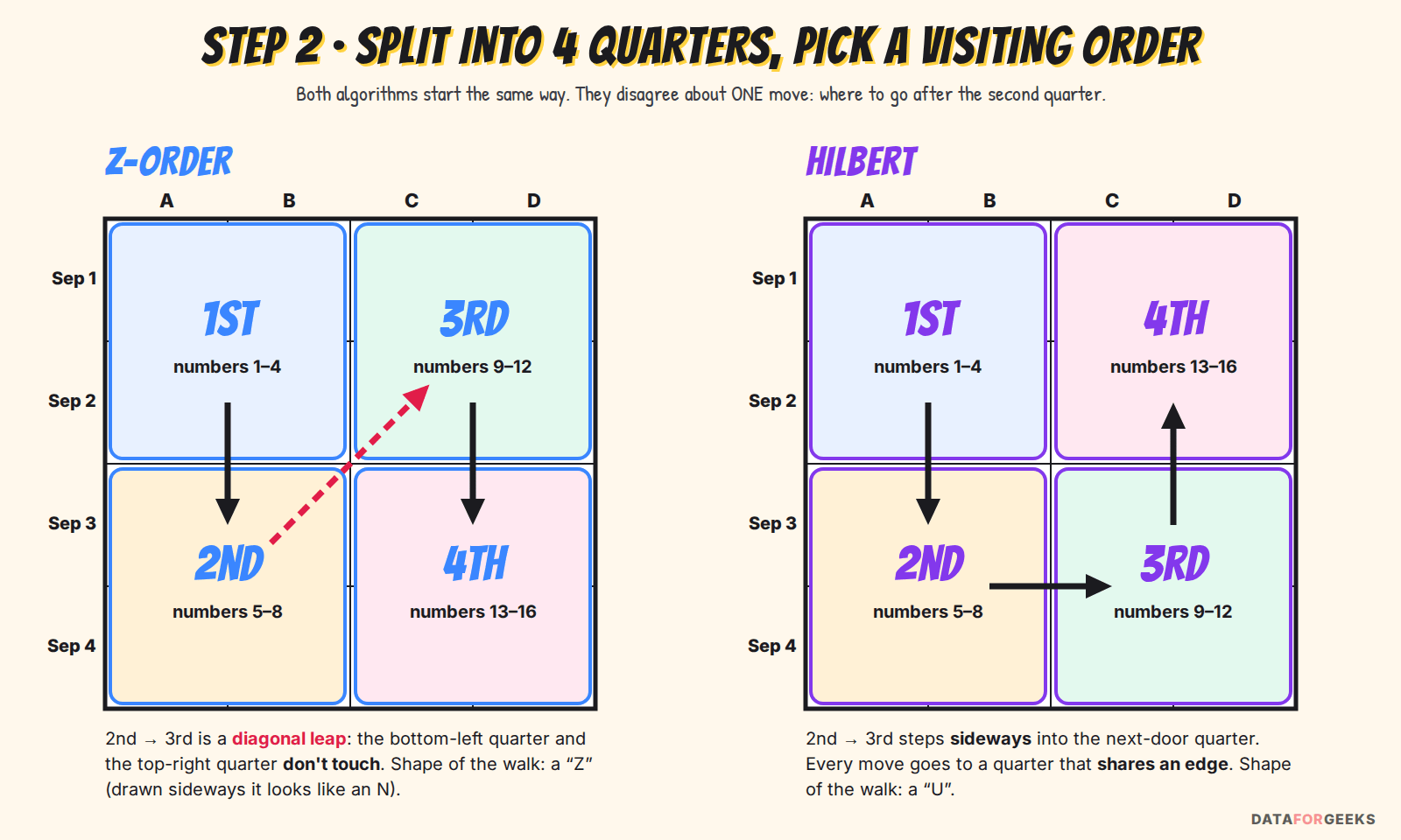
Both start in the top-left quarter (customers A–B, Sep 1–2) and both go down to the bottom-left quarter next. Then they disagree about one move:
- Z-order jumps diagonally to the top-right quarter. The bottom-left and top-right quarters don’t touch. That’s a leap.
- Hilbert steps sideways to the bottom-right quarter, the one right next door, and only then goes up.
Each quarter covers four squares, so each one “owns” a block of four numbers. Z-order gives numbers 9–12 to the top-right quarter; Hilbert gives it 13–16, because it gets there last.
Go one level deeper and number every square
Now repeat the trick inside each quarter: four squares, visit them in some order. Here’s where Hilbert’s one extra rule comes in.
- Z-order draws the same little shape in every quarter: top-left, bottom-left, top-right, bottom-right (a small “N”). Always the same way round, whether or not it lines up with the next quarter.
- Hilbert draws a little “U”, but turns or mirrors it so that it starts next to where the previous quarter ended and finishes next to where the next quarter begins.
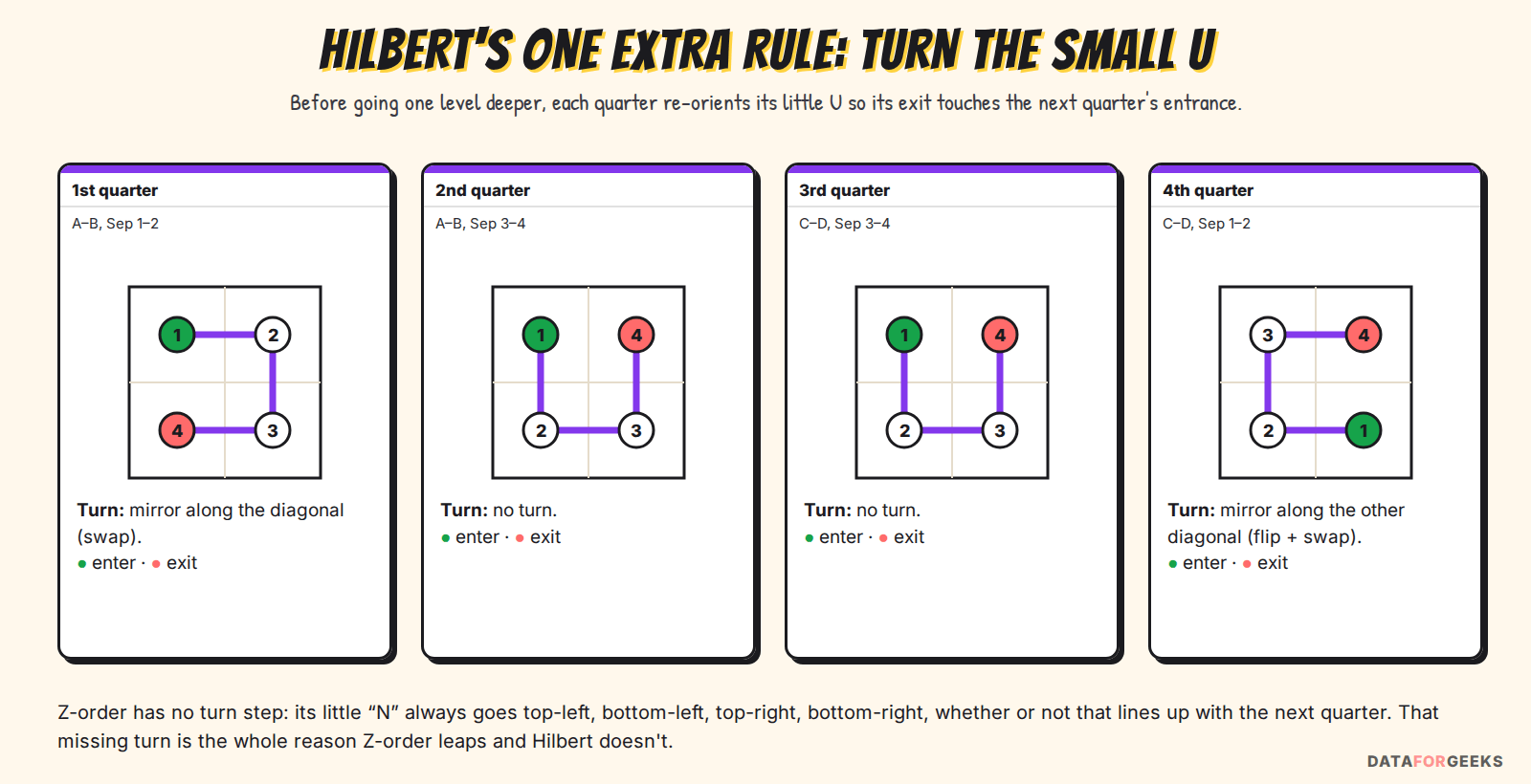
Put both levels together and every square gets its number:
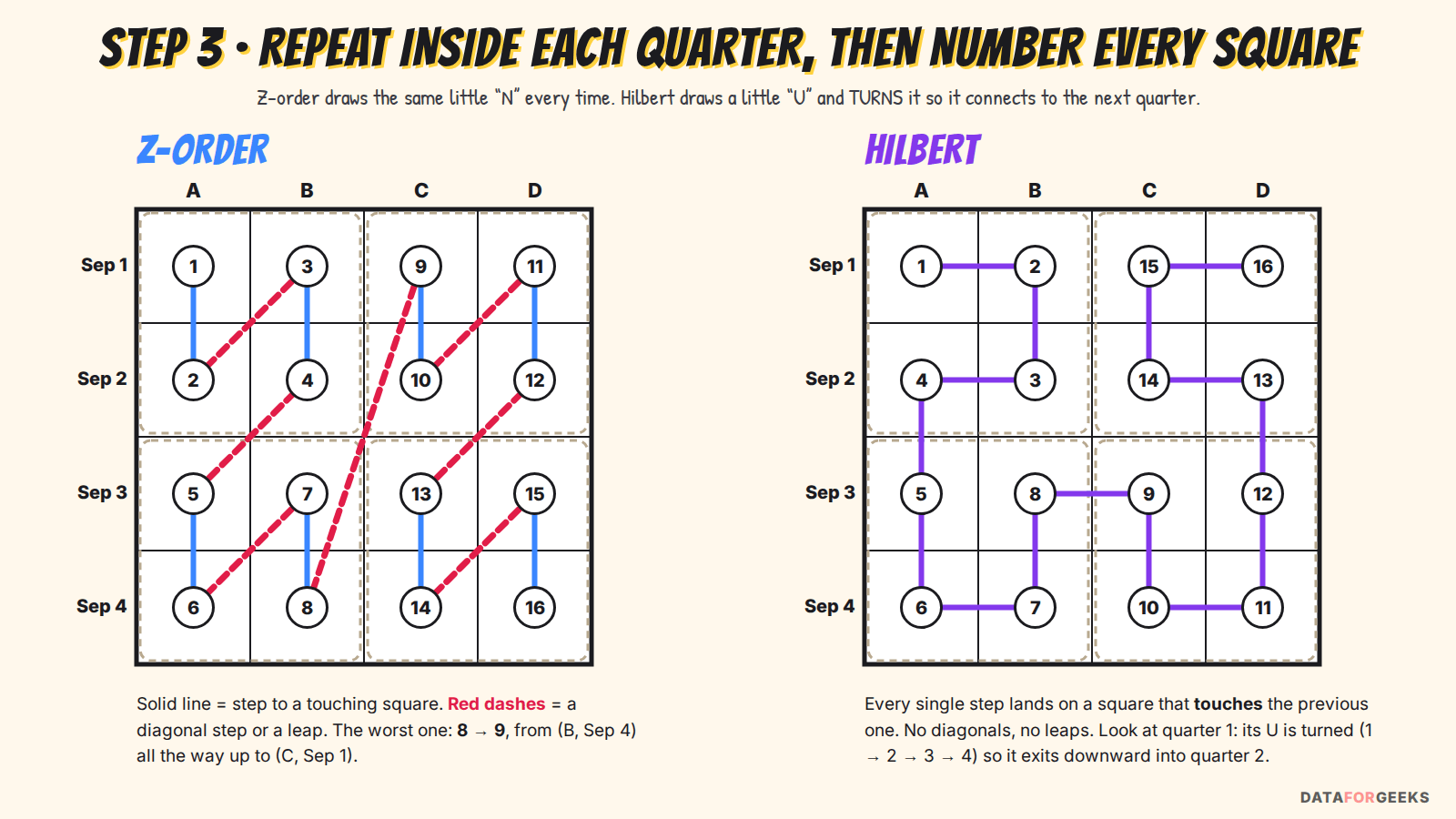
Trace the numbers 1, 2, 3… with your finger. That’s the best way to make it stick:
- Z-order mostly moves to nearby squares, but it moves diagonally often (1 → 2 is fine, 2 → 3 is diagonal) and sometimes leaps. The worst one is 8 → 9: from customer B on Sep 4 all the way to customer C on Sep 1.
- Hilbert never does either. Every single step lands on a square that shares an edge with the previous one.
💡 Tip: Remember it as three words each. Z-order: quarter, square, leap. Hilbert: quarter, square, turn. The turn is what removes the leap.
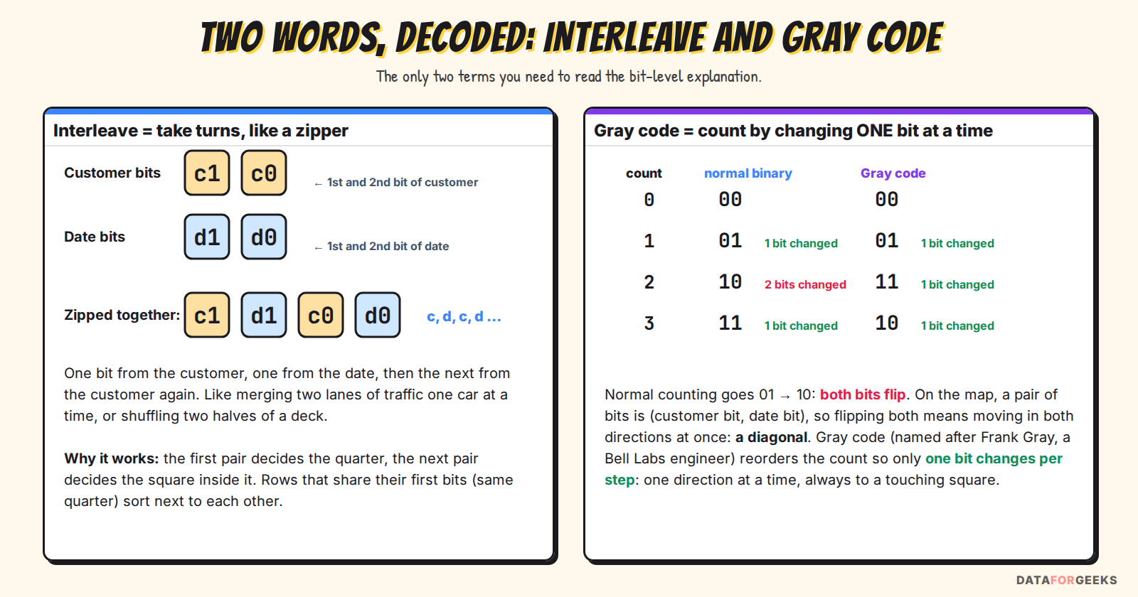
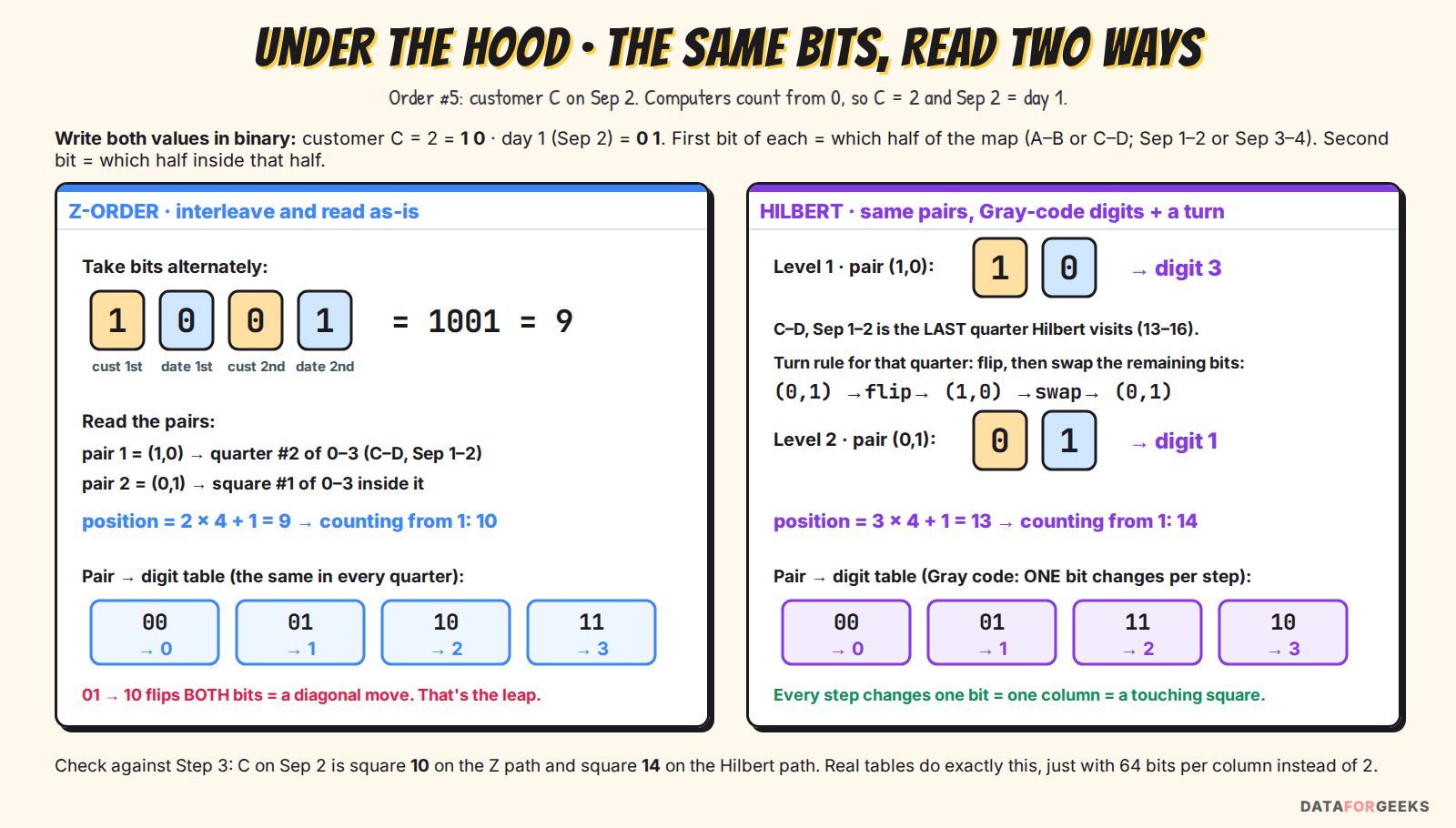
Sort the rows and fill the files
Now the payoff. Every row simply inherits the number of its square. Order #5 (C, Sep 2) gets 10 under Z-order and 14 under Hilbert. Then, for both algorithms:
- sort all rows by their number;
- fill files in that order: the first 6 rows into File 1, the next 6 into File 2, and so on;
- write each file’s label (min and max of each column);
- throw the numbers away. They are never stored.
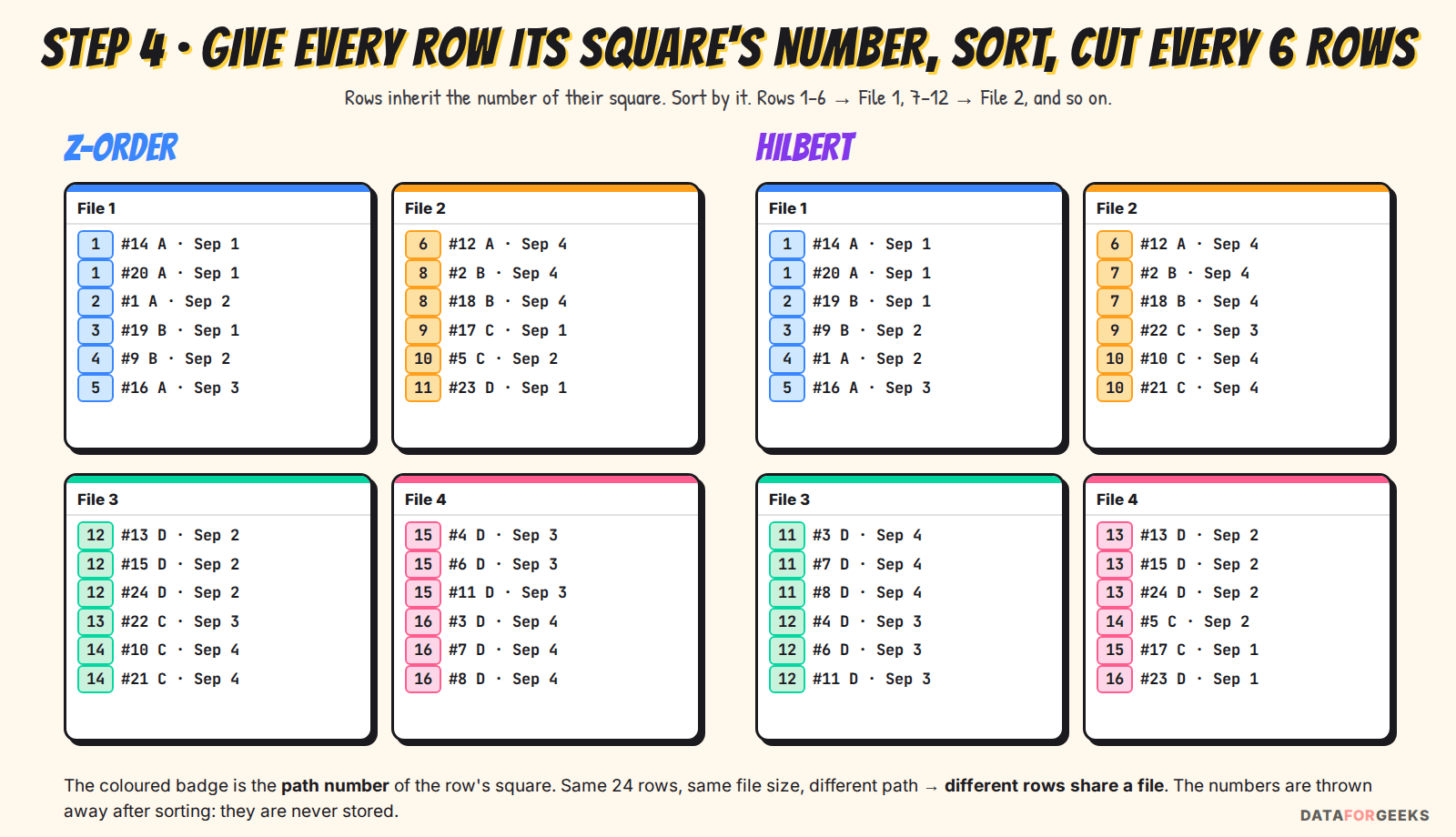
Same 24 rows, same file size, different path, so different rows end up sharing a file. Here’s where each file lands on the map, and what its label says:
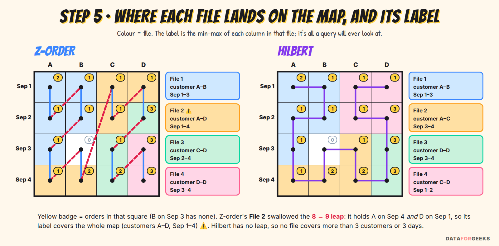
| File | No clustering | Z-order label | Hilbert label |
|---|---|---|---|
| 1 | A–D, Sep 2–4 | A–B, Sep 1–3 | A–B, Sep 1–3 |
| 2 | A–D, Sep 2–4 | A–D, Sep 1–4 ⚠️ | A–C, Sep 3–4 |
| 3 | A–D, Sep 1–4 | C–D, Sep 2–4 | D only, Sep 3–4 |
| 4 | A–D, Sep 1–4 | D only, Sep 3–4 | C–D, Sep 1–2 |
Look at Z-order’s File 2. It holds path numbers 6 to 11, and the 8 → 9 leap sits right in the middle. So it contains customer A on Sep 4 and customer D on Sep 1, and its label stretches across the whole map. One leap inside one file, and that file becomes useless for pruning. Hilbert has no leap, so none of its files covers more than three customers or three days.
YOU MIGHT BE WONDERING
What if a file boundary falls in the middle of a square?
It happens all the time in real tables: files are cut by size, not by squares. The rows of that square simply end up in two neighbouring files. It doesn’t change anything we’ve said: both files still cover a stretch of the path, and their labels are only wide if that stretch contains a leap. (In our small example I picked counts so each file boundary falls between squares, to keep the pictures clean.)
What happens when a query arrives
Here’s the part that surprises people: the query engine never sees the path. It doesn’t know or care whether the files were written with Z-order, Hilbert or no clustering at all. It does exactly one thing: compare its filter with each file’s label, skip what can’t match, and open the rest.
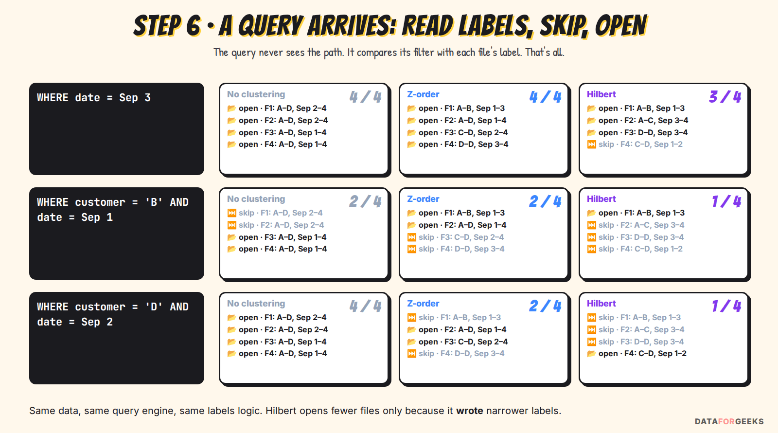
| Query | No clustering | Z-order | Hilbert |
|---|---|---|---|
| date = Sep 3 | 4 of 4 | 4 of 4 | 3 of 4 |
| customer = C | 4 of 4 | 2 of 4 | 2 of 4 |
| customer = B and date = Sep 1 | 2 of 4 | 2 of 4 | 1 of 4 |
| customer = D and date = Sep 2 | 4 of 4 | 2 of 4 | 1 of 4 |
The same check repeats one level down: inside each Parquet file, every row group (a chunk of rows) carries its own min/max, so a well-clustered file lets the reader skip row groups too.
So, to answer the most common confusion in one line: writing is where the two algorithms differ; reading is identical. Hilbert opens fewer files only because it wrote narrower labels.
Z-order vs Hilbert curve, side by side
| Stage | Z-order | Hilbert curve |
|---|---|---|
| Columns you name | 2–4 filter columns | Same |
| Core idea | Path through the map; neighbours on the path share a file | Same |
| Top-level quarter order | Z/N shape: includes a diagonal leap | U shape: every move to a touching quarter |
| Inside each quarter | Same small shape every time | Small U, turned to connect to the next quarter |
| In bits | Interleave the bits (take one from each column in turn) and read them as-is | Interleave, then read each pair in Gray-code order (one bit changes per step) and turn at each level |
| Leaps | Yes, and longer at every level | Never |
| Cost to compute | Very cheap | A few more bit operations per row; the sort costs the same |
| What’s stored | Files and their min/max labels | Same (the path number is thrown away) |
| How queries read | Compare filter with labels, skip, open | Exactly the same |
🧊 My take: The picture that finally made this click for me was the courier with the bag labelled “streets A–D, lanes 1–4”. Z-order isn’t a bad idea: it’s the right idea with an occasional long jump, and every jump that lands inside a file ruins that file’s label. Hilbert is the same idea without the jumps. That’s why I think Hilbert becoming available in Iceberg matters more than the size of the change suggests.
Z-order clustering in Iceberg: the first answer, and its crack
How bit interleaving works

Z-order clustering sorts rows by a key made from interleaving the bits of several columns, so rows close on all of those columns tend to land in the same files. Iceberg has supported zorder(...) for years. It’s exactly the path you just followed on the 4×4 map, done with bits: write each column’s value in binary, then interleave the bits (take turns: one from x, one from y, one from x, and so on). Sorting rows by that combined number keeps rows that are close in both columns mostly close on disk. Iceberg first converts each value (a date, a string, a number) into an order-preserving byte form, so it works across column types.
The crack: occasional big jumps

You saw the 8 → 9 leap on our 4×4 map. On bigger grids the same thing happens at every level. Walk the grid in Z-order and most steps are short, but at the boundary between big blocks the path leaps from one side of the space to the other. On the 8×8 grid above, the longest Z-order step spans 8 cells, and 49% of steps don’t land on a touching cell. On a 1024×1024 grid the longest step spans 1,024 cells.
Why does that matter? Files are written by cutting the sorted rows into chunks. When a chunk contains one of those jumps, it gets rows from two distant regions, and its min/max range stretches to cover both. Wider ranges mean more files overlap your filter, so more files get opened.
YOU MIGHT BE WONDERING
So is Z-order bad?
Not at all. Z-order is far better than a plain sort when you filter on several columns, and it’s cheap to compute. A Hilbert curve is a refinement of the same idea that removes Z-order’s one structural weakness. If your Iceberg version doesn’t have hilbert(...) yet, keep using zorder(...).
What is a Hilbert curve? The same idea, with no jumps

How a Hilbert curve is built

A Hilbert curve is a space-filling curve: a single continuous line that visits every cell of a grid exactly once, always stepping to an adjacent cell. Sorting rows by their position along it keeps rows that are close on several columns close together on disk.
Described by David Hilbert in 1891, it’s a single line folded so tightly that it passes through every cell of a grid, never crossing itself and never jumping. You build it recursively: start with a U through four cells, then replace each cell with a smaller U, rotated so the pieces join end to end, and repeat. Each row’s position along that line becomes its sort key, in place of Z-order’s interleaved bits. The same construction works for three, four or more columns.
If you like to see the mechanics, here’s the classic two-column version in Python. It’s the “quarter, square, turn” rule from the worked example: (3 * rx) ^ ry is the Gray-code digit, and the swap/flip is the turn.
Note: the code in this post was written with the help of Claude (an AI assistant) to clarify the ideas. It’s illustration, not production code.
def hilbert_index(x: int, y: int, bits: int) -> int:
    """Position of cell (x, y) along a Hilbert curve on a 2^bits x 2^bits grid."""
    n = 1 << bits
    d, s = 0, n >> 1
    while s > 0:
        rx = 1 if x & s else 0
        ry = 1 if y & s else 0
        d += s * s * ((3 * rx) ^ ry)
        if ry == 0:                      # rotate the quadrant so the pieces join up
            if rx == 1:
                x, y = n - 1 - x, n - 1 - y
            x, y = y, x
        s >>= 1
    return d

# 2x2 grid: (0,0) -> 0, (0,1) -> 1, (1,1) -> 2, (1,0) -> 3  (a U shape)
What “no jumps” does and doesn’t guarantee
It’s easy to oversell this, so let’s be precise:
- Guaranteed: rows that are next to each other in the sort order are neighbours in the data space. A file is a contiguous run of sorted rows, so every file stays in one compact region.
- Not guaranteed: that every pair of neighbours in the data space ends up close in the sort order. No curve can do that; a few boundaries always split close points apart.
For pruning, the first property is the one that counts, and it’s why Hilbert-clustered files have tighter ranges.
Scaling up to millions of rows
Our map had 4 customers and 4 days, so two levels of quarters were enough. A real table might have a million customers and five years of dates. What changes? Only the number of levels.
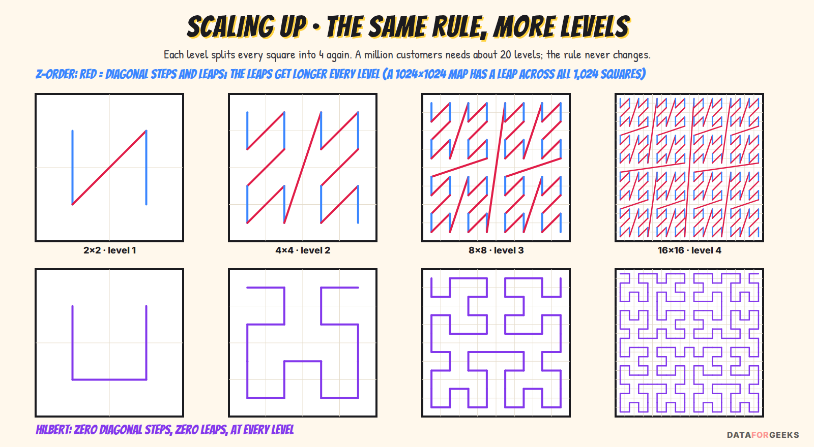
- More levels, same rule. Each level splits every square into four again. A million customers needs about 20 levels (220 ≈ 1 million); 1,826 days needs 11. The quarter-then-square logic never changes.
- Each square holds many rows. At the deepest level a square might be one customer on one day, holding dozens of orders. They all get the same number and travel together.
- Each file covers a stretch of the path. A 512 MB file might hold millions of consecutive rows along the path. On the map, that stretch is a blob. The more compact the blob, the narrower the label.
- Z-order’s leaps get bigger. On a 1,024 × 1,024 map, the longest Z-order jump crosses all 1,024 squares, and every file boundary near a leap produces a wide label. Hilbert’s longest step is still one square.
- The cost is the sort, not the key. Each row’s key is a few bytes and lives only during the rewrite. The expensive part is sorting (a shuffle) all the rows being rewritten, which is the same for both algorithms.
Hilbert vs Z-order: a simulation with a million rows
Diagrams are nice; numbers are better. I wrote a short Python simulation of exactly this mechanism. It isn’t a benchmark of Iceberg itself; it isolates the idea.
- Data: 1,000,000 rows with two filter columns, x and y, each on a 0–1023 scale. 70% are spread evenly and 30% sit in six hot spots, like busy dates or big customers.
- Layouts: the rows are sorted three ways (plain
ORDER BY x, y, Z-order and Hilbert), then cut into 64 equal files, keeping each file’s min and max per column, the same statistics Iceberg keeps. - Queries: 2,000 random range filters per workload: small and large boxes on both columns, x only, and y only. A file counts as opened if its ranges overlap the filter.
Note: the simulation code below was written with the help of Claude (an AI assistant) to clarify the ideas. It’s illustration, not production code.
Here is the code, one mechanism per block. Each one is just a key function: sort the rows by it and you get that layout. Paste all five blocks, in order, into one file and it reproduces the results table below in about a second (it only needs NumPy).

The picture explains the results before you see them. A plain sort produces thin, full-height slices: perfect for x, useless for y. Z-order produces blocks that serve both columns, but files that straddle a jump cover more space. Hilbert’s files are compact on both columns. Across 64 files, the average file covered 2.2% of the space with Hilbert versus 4.2% with Z-order. Roughly half the area means roughly half the chance of overlapping a random filter.

| Workload | ORDER BY x, y | Z-order | Hilbert | Hilbert vs Z-order |
|---|---|---|---|---|
| Filter on both, small box (5% × 5%) | 4.3 | 4.1 | 2.5 | −39% |
| Filter on both, large box (20% × 20%) | 14.4 | 10.4 | 7.8 | −25% |
| Filter on x only (5%) | 4.2 | 13.6 | 12.7 | −7% |
| Filter on y only (5%) | 64.0 | 18.0 | 12.4 | −31% |
Average files opened per query, out of 64. I re-ran it with two other random seeds and the numbers moved by less than 0.6 files.
Three lessons:
- Hilbert beat Z-order on every workload, by 25–39% on two-column filters.
- A plain sort is still best if you only ever filter on one column. Multi-column clustering is a trade: each column gives up a little so that all columns do well.
- The worst case is what hurts. The plain sort opened all 64 files for a y filter. Both curves avoid that cliff; Hilbert does it with tighter files.
🧊 My take: A 25–39% cut in files opened doesn’t sound dramatic, until you remember it applies to every query, every day, in every engine that reads the table. Layout improvements are the kind of saving nobody celebrates, but everyone sees in the monthly bill.
Real tables will differ: more columns, strings and timestamps, skewed data. Treat these as directional numbers and measure on your own table: cluster one copy with zorder and one with hilbert, then compare scanned files for your ten most common queries.
Limitations of Z-order and Hilbert clustering
Both algorithms share most of their weaknesses. Knowing them is what separates “we turned on clustering” from “clustering works for us”.
When one column’s values spread much wider than the other’s
Interleaving takes one bit from each column, level by level, starting from the top. But what if one column simply has more bits? A customer id up to a million needs 20 bits; 1,826 days needs 11. For the first 9 levels, every date has a 0 at that level, so only the customer decides the order. The sort behaves almost like ORDER BY customer_id, and every file ends up containing every date.
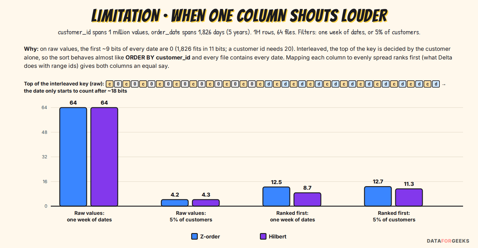
In the simulation, a one-week date filter opened all 64 files with both algorithms on raw values. After mapping each column to evenly spread ranks first, it dropped to 12.5 (Z-order) and 8.7 (Hilbert).
This is a real difference between table formats. Delta Lake’s clustering code first maps every column to one of 1,000 evenly filled “range ids” (by sampling the data), then interleaves those, so every column gets an equal say. Iceberg’s zorder(), and the new hilbert() which reuses the same encodings, work on each value’s own order-preserving bytes. What to do: cluster on columns with comparable spreads, or on a derived column that spreads evenly, and partition by time instead of clustering on it.
Every extra column dilutes the others
The key has a fixed amount of “closeness” to share. With two columns, each gets half the levels; with four, each gets a quarter. Filters on all clustered columns stay cheap, but filters on just one of them get steadily worse:
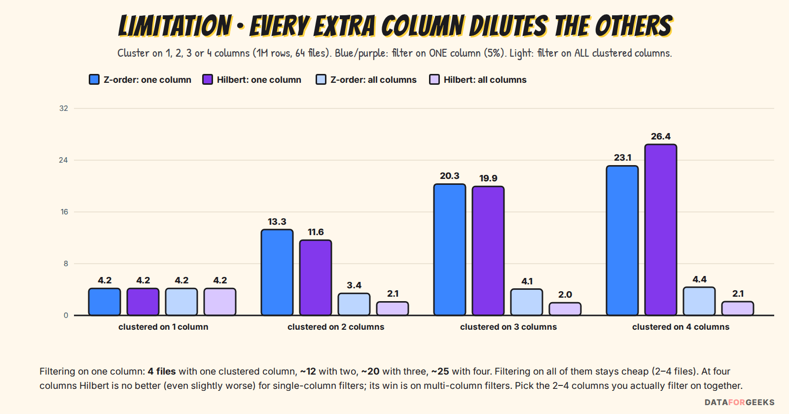
Notice the last group: at four columns, Hilbert is no better (slightly worse, in fact) than Z-order for single-column filters. Its advantage is on filters that combine columns. That’s also why Delta caps liquid clustering at 4 columns. Iceberg has no hard limit, but the same maths applies: pick the 2–4 columns you actually filter on together.
Hot values
If one customer owns 30% of all rows, those rows fill at least 19 of 64 files no matter what. In the simulation, a query for that one customer opened 26–27 of 64 files with either algorithm. That’s unavoidable: the data really is that big. Add a date filter, though, and clustering still helps: 4.9 files with Z-order, 3.6 with Hilbert. Inside a hot customer, all its bits are identical, so the other column decides the order, which is exactly what you want.
Long strings with a shared prefix
By default Iceberg uses only the first 8 bytes of a string column to build the key (the var-length-contribution option controls this). customer_000123 and customer_000456 look identical in their first 8 bytes, so that column contributes almost nothing. Cluster on a shorter, evenly spread code, or raise the setting.
Other things worth knowing
- Low-cardinality columns (status, country) waste levels. Partition by them instead, if they’re selective at all.
- Identity partition columns are ignored. Inside a partition they’re constant, so Iceberg drops them from the clustering columns with a warning.
- New data arrives unclustered. Files written after the last compaction have wide labels until the next run. Schedule compaction on recent partitions.
- It’s a rewrite. Clustering means reading, sorting and rewriting data. Scope it to the partitions that changed.
- Verify, don’t assume. Compare scanned vs skipped files before and after (the Spark UI’s SQL tab shows them; see my Spark UI guide), or inspect file bounds in Iceberg’s
filesmetadata table.
Beyond Hilbert: layouts that can do even better
Hilbert is the best built-in option for an Iceberg table today, but it isn’t the end of the road. It’s a fixed curve: it treats every column equally and ignores what your queries actually look like. The ideas below go further. Most are research or engine-specific features, so treat this as a map of where things are heading, not a to-do list.
| Technique | What it does better | Where it’s used |
|---|---|---|
| Rank first, then curve | Maps each column to evenly filled ranges before interleaving, so one wide column can’t dominate (the spread-skew problem above) | Delta Lake Z-order and liquid clustering (range ids) |
| Onion curve (2018) | A different fixed curve, proven near-optimal at keeping range-query results in few pieces; beats Hilbert for many query shapes | Research |
| Learned curves: BMTree, LMSFC (VLDB 2023) | Learn the curve’s shape from your data and past queries, instead of using one fixed pattern everywhere | Research prototypes |
| Workload-aware layout trees: Qd-tree (SIGMOD 2020) | Skip curves entirely: cut the data into blocks using the filters your queries actually run, so common queries hit very few blocks | Research (Microsoft Research and UC Berkeley); the idea behind “learned layouts” |
| Automatic clustering | The platform picks clustering keys from your query history (Databricks) or keeps the table clustered on your keys in the background (Snowflake) | Databricks automatic liquid clustering, Snowflake automatic clustering |
| Map cells: S2, H3 | Purpose-built grids for latitude/longitude; cluster on the cell id | Google S2 (numbers its cells along a Hilbert curve), Uber H3 (hexagons) |
The common thread: the more a layout knows about your data and your queries, the better it prunes, and the more it costs to build and maintain. A fixed curve like Hilbert is the sweet spot for an open table format today: no training, no query history needed, and every engine benefits.
Why Hilbert clustering in Apache Iceberg is exciting
Why I’ve been waiting for this

The first time I looked at Iceberg seriously, I was fighting append-only Snowpipe pipelines, with late-arriving data, reprocessing and duplicate compute. Iceberg promised a way out, but support was still early, so I stayed with what worked. I’ve watched it close one gap after another since then.
When I wrote my Iceberg deep-dive in 2025, I made two arguments that this change directly builds on:
- Metadata-driven pruning is Iceberg’s quiet superpower. I wrote that Iceberg “leverages manifest files and metadata layers to prune irrelevant data before reading.” Hilbert clustering makes exactly those per-file statistics sharper, so the same metadata now skips far more files.
- Partition evolution is the hidden superpower for layout. Partitions decide which part of a table a query touches. Clustering is the missing other half: how tightly rows are packed inside those partitions. Together they cover both levels of the layout.
My comparison of Delta, Hudi and Iceberg in that post focused on transactions, schema and partition evolution, and engine support. Data layout optimization was the one area where Iceberg was behind: Hudi and Delta already clustered with Hilbert curves, and Iceberg users had Z-order. That’s the gap this closes.
Three reasons it matters

Hilbert clustering isn’t new to open source: Apache Hudi has had it since 2021, and Delta Lake’s liquid clustering is built on it. What’s new is the Iceberg Hilbert curve option: native to the table format, and that matters more than it sounds:
- Iceberg is the format the most engines share. Spark, Trino, Flink, Snowflake, Athena, BigQuery, Dremio and others read Iceberg tables, and many write them too. The benefit of clustering lives in the table’s file statistics, so you cluster once and every engine that reads the table skips the same files. You don’t need a specific engine or vendor to get the speed-up.
- No format switch. Until now, Iceberg teams who wanted Hilbert-quality clustering had to switch table formats or rely on a vendor platform’s own optimizer. Now it’s one word in the compaction procedure they already run.
- It arrives with geospatial types. Iceberg 1.12 also wires through the geometry and geography types added in the V3 spec. Clustering on coordinates is what makes spatial filters prune well (more on that below).
Where you’ll meet these algorithms: Iceberg, Delta and Hudi
- Apache Iceberg:
zorder(...)in therewrite_data_filesprocedure today;hilbert(...)is expected in Iceberg 1.12, starting with Spark 4.1. The how-to section below shows how to use it. - Delta Lake:
OPTIMIZE … ZORDER BYuses Z-order; liquid clustering uses Hilbert, on up to 4 columns, with the range ids described above. - Apache Hudi: has offered both Z-order and Hilbert layout optimization since version 0.10 (2021).
The same idea shows up far beyond table formats: map tiles, spatial indexes and image processing all use space-filling curves. If you’ve read my ride-hailing data model post, pickup latitude and longitude are the textbook case: nearby pickups should live in the same file.
What becomes possible with Hilbert clustering

One table for many query patterns
Back to our events table, and the most immediate win of the Iceberg Hilbert curve. Instead of choosing between date and customer, or keeping two copies, you cluster on both: hilbert(event_date, customer_id). Dashboards filtering by date, support looking up a customer, and analysts asking for one customer over one month all prune well from the same table. Fewer copies means less storage, fewer pipelines to keep in sync, and one source of truth.
A real geospatial lakehouse

Dates and IDs at least have an order. Map coordinates don’t: there’s no meaningful answer to “is Paris bigger than Tokyo?”. Sort a trips table by longitude and cities at the same longitude but different latitudes end up in the same files, so spatial filters prune poorly.
A Hilbert curve gives the map a locality-preserving order: nearby points get nearby positions, so each file becomes something like a compact map tile. Think of the trips table from my ride-hailing data model post. Clustered on pickup latitude and longitude (plus time), “all pickups in this neighbourhood last Friday” opens a handful of tiles instead of the whole city. Delivery zones, fleet telemetry, store footfall and IoT sensors all have the same shape of question. Combined with Iceberg’s new geometry types, this is what makes geospatial analytics on an open lakehouse practical.
Fast entity-plus-time lookups
“Show me everything this customer, device or account did between these dates” is one of the most common questions in data engineering. It powers customer 360 views, support tools, fraud investigations and feature tables for ML. With hilbert(entity_id, event_time), both halves of the filter prune, so these lookups become fast without a separate index or a copy sorted by entity.
Cheaper, snappier dashboards
BI dashboards are multi-column filters by nature: date, region, product, channel. Every file a dashboard query doesn’t open is money you don’t spend and seconds your users don’t wait. Tighter files also mean fewer rows decoded once a file is opened, because Parquet row groups inside it are clustered too (see why Parquet beats CSV on cost).
Clustering that travels between engines
Today the clustering choice lives in your compaction job: you pass 'hilbert(c1, c2)' when you run it. The Iceberg community is now discussing the next step for the V4 table spec: storing the clustering definition itself in table metadata, with every parameter spelled out, for example per-column scaling so mixed types use the curve well. If that lands, any engine could read the table’s clustering intent and keep the layout up to date, not just the job that wrote it. That’s the path toward automatic, “liquid” clustering in a fully open format. It’s still under discussion, but it’s the right direction.
How to use the Iceberg Hilbert curve in rewrite_data_files
Once you’re on Iceberg 1.12 with Spark 4.1 (Spark 4.0 support is planned), switching to the Iceberg Hilbert curve is one word in the rewrite_data_files procedure:
-- what you may run today
CALL catalog.system.rewrite_data_files(
  table      => 'db.events',
  strategy   => 'sort',
  sort_order => 'zorder(event_date, customer_id)'
);

-- with Hilbert clustering
CALL catalog.system.rewrite_data_files(
  table      => 'db.events',
  strategy   => 'sort',
  sort_order => 'hilbert(event_date, customer_id)',
  options    => map('rewrite-all', 'true')   -- first run: re-cluster every file
);
Practical tips:
- Pick 2–4 columns that your queries filter on most. Every extra column dilutes the clustering of the others.
- Re-run on a schedule. New data arrives unclustered, so run compaction nightly or weekly on recent partitions.
- Filter on the raw clustered columns. Pruning uses each column’s stored min/max, so
WHERE event_date = …prunes, while filters on expressions the engine can’t map back to the column may not. - Expect a little more CPU at write time. Computing a Hilbert position costs slightly more than interleaving bits. You pay it once during compaction, and every read afterwards benefits.
- Watch long strings. Iceberg’s curve encodings only look at the first few bytes of variable-length values (
var-length-contribution, default 8 for Z-order), so strings with long common prefixes, such as URLs, won’t cluster well with either curve. - Measure before you switch. Try it on a copy or a few partitions and compare scanned files for your common queries.
YOU MIGHT BE WONDERING
Does this replace partitioning?
No. Partitioning, for example by day, decides which partitions a query plans over at all; clustering decides how tightly rows are packed within those partitions. They work together: partition coarsely by time, then Hilbert-cluster inside each partition on the columns you filter by. If you’re new to Iceberg, my Iceberg introduction covers partitioning and metadata.
Summary: Hilbert vs Z-order in Apache Iceberg
Key takeaways
- Fast queries on big tables come from skipping files, and that needs each file to have a narrow min/max label.
- A plain sort helps one column and can be useless for the others (64 of 64 files in my simulation).
- Z-order and Hilbert share one method: place rows on a map, number the squares along one path (quarter first, square second), sort, fill files in order.
- The difference is only the path. Z-order reads the interleaved bits as they are and sometimes leaps; Hilbert reads the same bits in Gray-code order, turns the small U at every level, and never leaps.
- Reading is identical. Queries only compare filters with labels. Hilbert wins by writing better labels: 25–39% fewer files opened than Z-order for two-column filters in my simulation.
- The limits are shared: mismatched column spreads, too many columns, long shared string prefixes, and single-column workloads where a plain sort wins.
- Having it inside Iceberg is the real news: cluster once, and every engine that reads the table benefits, with no format switch.
- It unlocks new designs: one table instead of many copies, geospatial analytics on an open lakehouse, fast entity-plus-time lookups and cheaper dashboards.
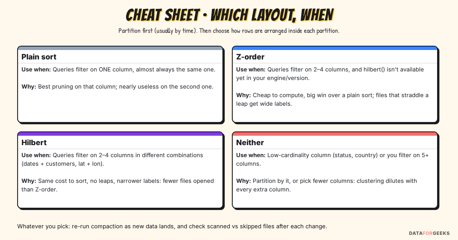
Cheat sheet: plain sort vs Z-order vs Hilbert
| Plain sort | Z-order | Hilbert | |
|---|---|---|---|
| Best for | One dominant filter column | 2–4 filter columns | 2–4 filter columns, geospatial |
| How the key is built | Column values in order | Interleaved bits | Position along a folded curve |
| Jumps between consecutive rows | Wraps at every new value of the first column | Occasional, large | None |
| File ranges | Narrow on the first column only | Good on all, wider at jumps | Tight on all |
| Iceberg syntax | 'x ASC, y ASC' | 'zorder(x, y)' | 'hilbert(x, y)' (1.12+, Spark 4.1) |
The part that excites me
For years, “sort your table” meant “pick a winner”. The Iceberg Hilbert curve quietly retires that trade-off for most tables, and it does so in the open format every major engine already speaks. The idea is from 1891. Having it one word away, in a table format anyone can use, is what’s new.
In May 2025 I ended my Iceberg post with a slightly provocative line: “If you’re not already using Iceberg — you’re building on yesterday’s architecture.” Sixteen months later, I’d keep it and add one more: if you’re already on Iceberg, it’s time to look at how your data is laid out, not just where it’s stored. Hilbert clustering is the easiest place to start.
And if you remember one sentence from the worked example, make it the courier’s: same parcels, same bags, one route leaps.
Are you clustering with zorder today? Tell me in the comments which columns you cluster on and which query patterns you’d like to speed up. If you test hilbert once 1.12 lands, I’d love to see your scanned-files numbers.
Frequently asked questions
What is Iceberg Hilbert curve clustering?
Iceberg Hilbert curve clustering is a sort order for Iceberg’s rewrite_data_files procedure that arranges rows by their position along a Hilbert curve across several columns. Rows that are close on all of those columns end up in the same data files, so each file covers a narrow range and queries can skip more files.
How is a Hilbert curve different from Z-order?
Both give every row a single position number built from several columns, then sort rows by it so that rows with similar values land in the same file. Z-order reads the interleaved bits as they are, so its path sometimes leaps across the data space. A Hilbert curve reads the same bits in Gray-code order and turns the path at every level, so every step moves to a touching cell and it never leaps.
Why is Hilbert clustering in Iceberg a big deal?
Iceberg is the table format the most query engines share. Clustering improves the table’s own file statistics, so you cluster once and Spark, Trino, Flink, Snowflake, Athena and other engines that read the table all skip the same files, without switching formats or vendors.
Which Iceberg version supports hilbert() in rewrite_data_files?
It is expected in Apache Iceberg 1.12, starting with Spark 4.1, with Spark 4.0 support planned. Until then, zorder() is the multi-column option.
How do I use Hilbert clustering in Iceberg?
Call rewrite_data_files with strategy ‘sort’ and sort_order ‘hilbert(col1, col2)’, exactly as you would with ‘zorder(col1, col2)’. Pick the 2 to 4 columns your queries filter on most, and re-run compaction regularly as new data arrives.
Is Hilbert always better than Z-order?
No. For filters that combine several clustered columns it usually prunes better; in our simulation it opened 25 to 39 percent fewer files than Z-order, at the same sorting cost. But if nearly every query filters on one column, a plain sort is still best, and for single-column filters on a table clustered by many columns Hilbert can be equal or slightly worse. Both share the same limitations: skewed spreads, long string prefixes, hot values and data written after the last compaction. Measure on your own tables before switching.
Does Hilbert clustering help geospatial queries?
Yes, that is one of its biggest use cases. Coordinates have no natural one-dimensional order, and a Hilbert curve gives nearby points nearby positions, so files behave like compact map tiles that spatial filters can skip.
Does clustering replace partitioning in Iceberg?
No. Partitioning decides which parts of the table a query plans over, while clustering decides how tightly rows are packed within them. A common pattern is to partition coarsely by time and then Hilbert-cluster inside each partition on the columns you filter by.
What is file pruning (data skipping) in Iceberg?
Iceberg stores the minimum and maximum value of each column for every data file. When a query filters on a column, the engine skips every file whose range cannot contain matching values, without opening it. Clustering with Z-order or Hilbert curves makes those ranges narrower, so more files are skipped.
Why does a Hilbert curve prune more files than Z-order?
Files are filled with consecutive rows along the path. When a file contains one of Z-order’s leaps, it holds rows from two distant regions and its min/max label stretches over both. Hilbert has no leaps, so its files cover compact regions with narrow labels, and queries can skip more of them. In a million-row simulation Hilbert opened 25 to 39 percent fewer files than Z-order on two-column filters.
Does the query engine need to know whether Z-order or Hilbert was used?
No. Reading is identical. The engine only compares the query filter with each file’s min/max statistics and skips files that cannot match. Z-order and Hilbert only change which rows were written into each file, and therefore how narrow those statistics are.
Is the Z-value or Hilbert value stored in the table?
No. The position number is computed for each row during the rewrite, used to sort the rows, and then thrown away. Only the data files and their per-column min/max statistics are kept.
Does Z-order or Hilbert clustering build a huge matrix of all value combinations?
No. The map is only a way to picture the idea. The computer calculates one small number per existing row from the bits of its values. Work and storage grow with the number of rows, not with the number of possible combinations.
How many columns should I use for Z-order or Hilbert clustering?
Usually 2 to 4, chosen from the columns your queries filter on together. Every extra column dilutes the clustering of the others: in a simulation, a filter on one column opened about 4 of 64 files with one clustered column, about 12 with two, about 20 with three and about 25 with four. Delta Lake’s liquid clustering allows at most 4 clustering columns; Iceberg has no hard limit.
What happens if one column has a much wider range of values than another?
The column with more bits decides the top of the sort key on its own, so clustering behaves almost like a plain sort on that column. In a simulation with customer ids up to a million and five years of dates, a one-week date filter opened every file. Delta Lake avoids this by mapping each column to evenly filled range ids first; Iceberg’s zorder and hilbert work on each value’s own bytes, so choose columns with comparable spreads or cluster on an evenly spread derived column.
When is a plain sort better than Z-order or Hilbert?
When nearly all queries filter on one column. A plain sort gives the narrowest possible ranges on that column. Z-order and Hilbert trade some of that away to also help other columns, which only pays off if you filter on them.
Further reading on DataForGeeks:
- Apache Iceberg: the data lake breakthrough reshaping big data
- One Ride, 400 Milliseconds: a ride-hailing data model
- How to debug a slow Spark job and fix data skew
- Cost and performance analysis: CSV vs Parquet
- Apache Spark performance tuning and best practices
