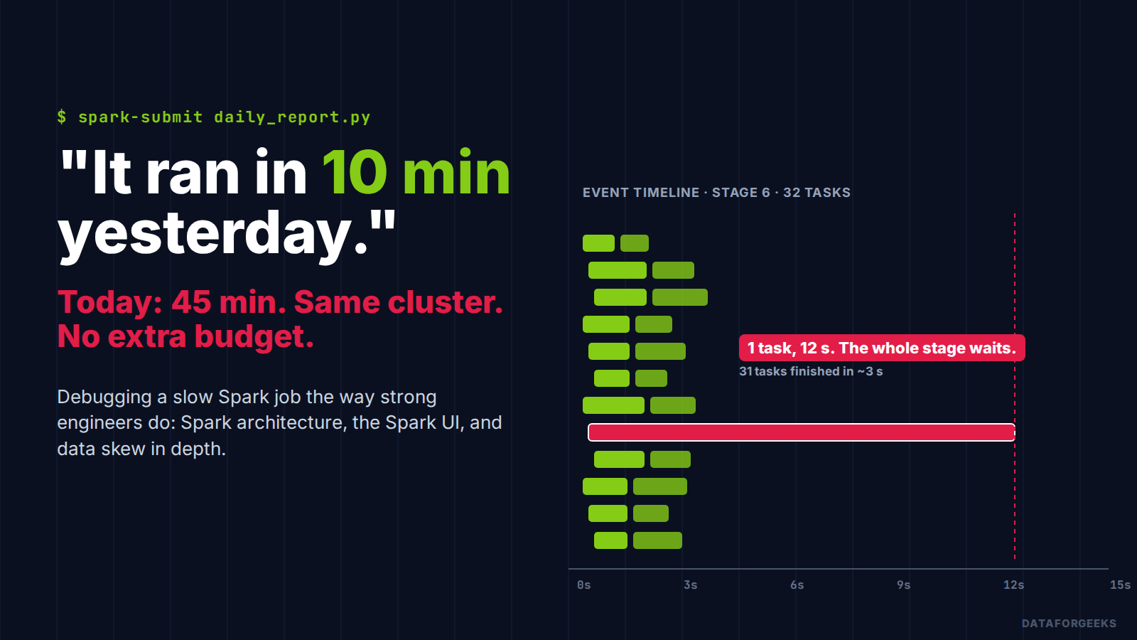
It Ran in 10 Minutes Yesterday: How to Debug a Slow Spark Job and Fix Data Skew

“It ran in 10 minutes yesterday. Today it takes 45.” Every data engineer has read that message at 9 a.m., and interviewers know it. The question sounds like a small follow-up after a big design round, but it quietly tests almost everything: how Spark actually runs your code, whether you can read the Spark UI, whether you know what data skew looks like, and whether you fix things with evidence or with a bigger credit card.

This post shows how to debug a slow Spark job the way a strong senior data engineer would, and how to explain it in an interview. Not as a list of tuning flags, but as a debugging story: how Spark runs your code, how to read the Spark UI, and how to find and fix data skew in Spark, with real Spark UI screenshots from a job we deliberately broke and then fixed four different ways.

By the end you’ll be able to:

• open your answer with a first line that sets the pace of the whole round;
• explain how Spark turns code into jobs, stages, shuffles and tasks, and why one task can hold up a whole stage;
• walk the Spark UI screen by screen and prove data skew with numbers;
• choose between AQE, broadcast, salting and hot-key isolation, and explain the trade-offs;
• rule out the other usual suspects and stop the problem from coming back.

Our candidate is Nikhil again (you may have met him in One Ride, 400 Milliseconds and The Vendor Who Pushes). Same system-design practice session with friends, second half of the round. The design is done; now the interviewer leans back and asks about Spark.

---

The question, and why most answers go wrong

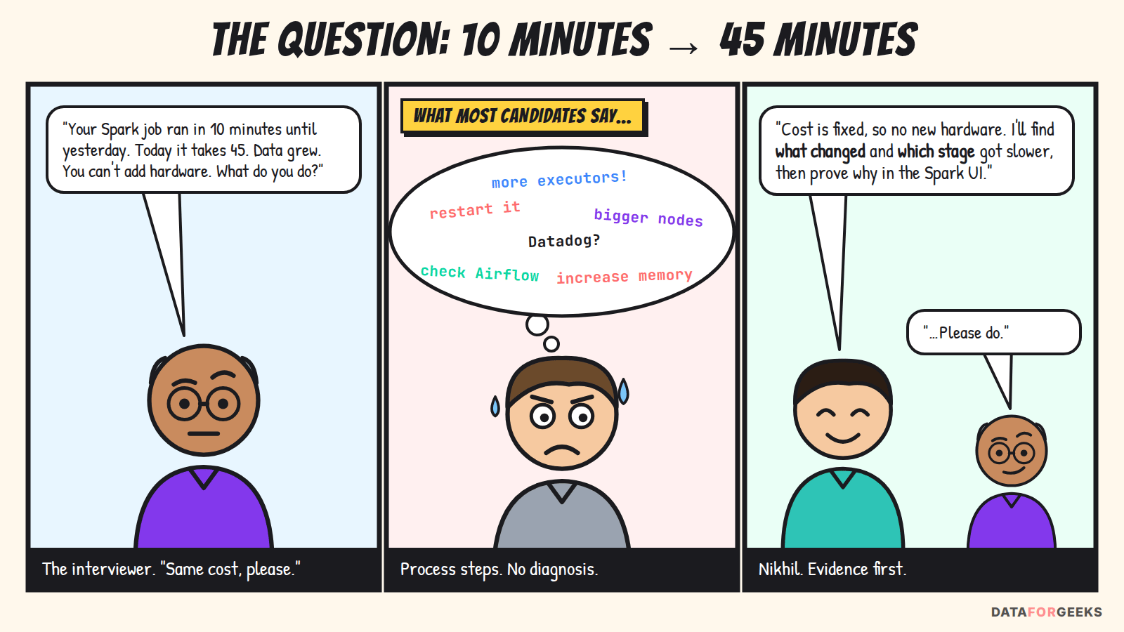
“Your daily Spark job has run in about 10 minutes for months. Since yesterday it takes 45. The data has grown. You’re not allowed to add nodes, bigger instances or any extra cost. How do you find out what’s wrong, and how do you fix it?”

Three constraints hide in that prompt, and each one closes a lazy exit:

• “Since yesterday”: something changed. Your first job is to find out what, not to start tuning.
• “The data has grown”: a tempting explanation, and often only half the story. If data grew 3× and runtime grew 4.5×, something non-linear is going on.
• “No extra cost”: “add executors” and “use bigger nodes” are off the table. You have to make the same hardware do the work better.

Here’s what interviewers are really scoring:

What they’re checking	Weak signal	Strong signal
Method	Jumps to a fix (“increase memory”)	A repeatable loop: change → stage → evidence → cause → fix → verify
Spark internals	“Spark is distributed”	Explains jobs, stages, tasks, shuffles and why one task can hold up a stage
Tooling	“I’d check the logs”	Knows which Spark UI tab answers which question
Skew	“Use salting”	Detects skew from task quantiles, then picks among AQE, broadcast, salting, splitting hot keys
Cost awareness	Adds hardware	Makes the same cluster faster and explains why that works
Prevention	Stops at the fix	Adds alerts and checks so it doesn’t happen again

The first 60 seconds: how to open your answer

Most candidates think the hard part of this question is Spark. It isn’t. The hard part is the first sentence, because it decides who leads the next 20 minutes. Open with a fix and you spend the round defending a guess. Open with a vague “I’d check the logs” and the interviewer takes over with their own checklist. Open with a clear, evidence-first plan and the interviewer tends to follow your agenda, which means you get to talk about the things you know best.

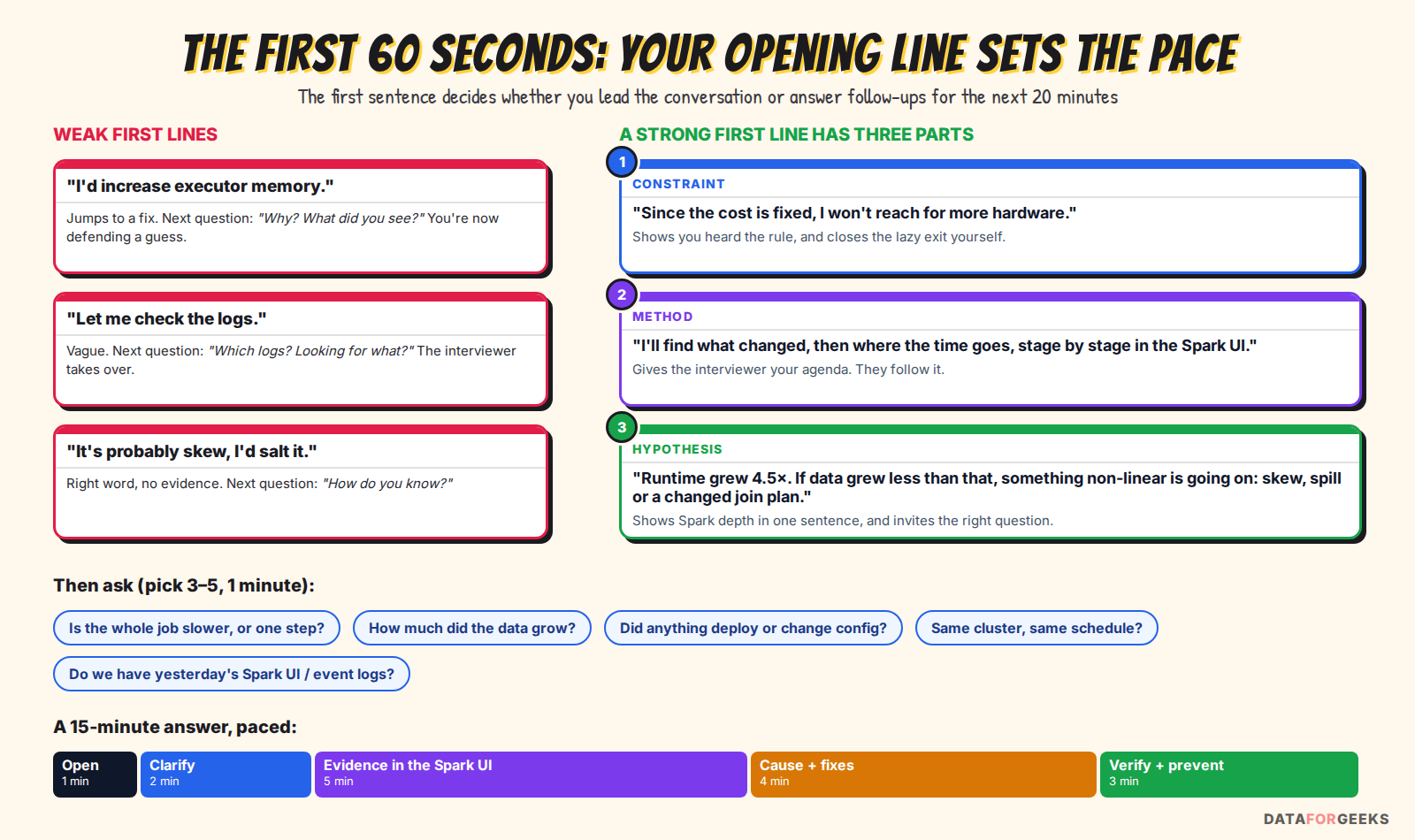
Here is how Nikhil opens. Read it out loud once; it takes about 20 seconds:

“Since the cost is fixed, I won’t reach for more hardware. I’ll first find out what changed and then where the time goes, stage by stage, in the Spark UI. One thing I’d check early: the runtime grew 4.5 times. If the data grew by less than that, something non-linear is going on, like data skew, spill or a join plan that changed, not just more volume.”

Three sentences, three jobs:

Part	What he says	What the interviewer hears
Constraint	“I won’t reach for more hardware.”	He listened. The lazy answer is off the table before they have to take it away.
Method	“What changed, then where the time goes, stage by stage.”	He has a process. I can let him drive.
Hypothesis	“4.5× time… non-linear… skew, spill or a changed join.”	He knows how Spark behaves. Let’s see if he can prove it.

Notice what he did not say: no tool names, no config flags, no “I would salt it”. The hypothesis is phrased as something to check, which keeps him honest if the evidence points elsewhere.

Then ask a few sharp questions

Right after the opener, spend about a minute on clarifying questions. Each one should be able to change your path:

Question	Why it matters
Is the whole job slower, or one step?	Narrows the search from the whole pipeline to one query or stage.
How much did the data grow?	3× data and 4.5× time is non-linear; 5× data and 4.5× time is just volume.
Did anything deploy, or any config change?	Code and config changes are the most common “since yesterday” causes.
Same cluster, same schedule, same neighbours?	Rules resource contention in or out.
Do we have yesterday’s Spark UI or event logs?	A good run to compare against is the fastest debugging tool there is.

In our practice session the interviewer answers: “One step, the daily report. The data roughly tripled. No deploy. Same EMR cluster. Yes, event logs are kept.” Nikhil now has his first clue: 3× data, 4.5× time.

Pace the rest of the answer

Say the plan once, then follow it: about 1 minute to open, 2 to clarify, 5 on evidence in the Spark UI, 4 on the cause and fixes, and 3 on verification and prevention. If the interviewer interrupts, answer and come back to the plan (“…so, back to the stage metrics”). That sentence alone shows you’re in control of the conversation.

How to answer: the six-step debugging loop

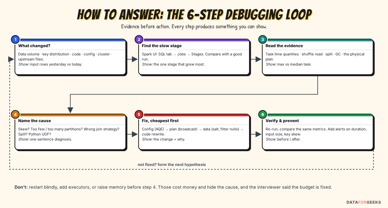
The opener promised a method; this is it. Every step produces something you can show the interviewer:

“I’ll check what changed between yesterday and today. Then I’ll open the Spark UI for both runs and find which stage got slower. Inside that stage I’ll look at the task metrics to tell volume from skew from spill. Once I can name the cause, I’ll fix it the cheapest way first (configuration, then the join strategy, then the data, then the code) and compare the same metrics after the fix.”

Step one deserves its own checklist, because “what changed?” has more answers than people expect:

What could have changed	How to check quickly	Typical effect
Input volume	Input size / rows in the Stages tab, or count() per day	Linear slowdown (3× data ≈ 3× time)
Key distribution	Top-N keys by count on the join / group key	One huge task, non-linear slowdown
Number and size of input files	File listing, “number of files read” in the SQL tab	Thousands of tiny tasks, slow listing
Code / query	Git history, the deployed version	New join, UDF, collect(), lost filter
Configuration	Environment tab, spark-defaults, job parameters	AQE or broadcast disabled, fewer partitions
Small table grew past a limit	Plan: BroadcastHashJoin yesterday, SortMergeJoin today	A cheap join became a full shuffle
Cluster / neighbours	Executors tab, YARN / cluster metrics, spot interruptions	Fewer executors, lost nodes, retries
Upstream data quality	Null / default keys, duplicates	Join explosion, a giant “NULL” partition
File format / compression	A new large .gz or other non-splittable file	One input task reads the whole file

Spark architecture in ten minutes

You can’t read the Spark UI without a mental model of what Spark is doing, and interviewers often probe it here (“what’s a stage?”). This is the minimum you need, explained with our job.

Driver, cluster manager and executors

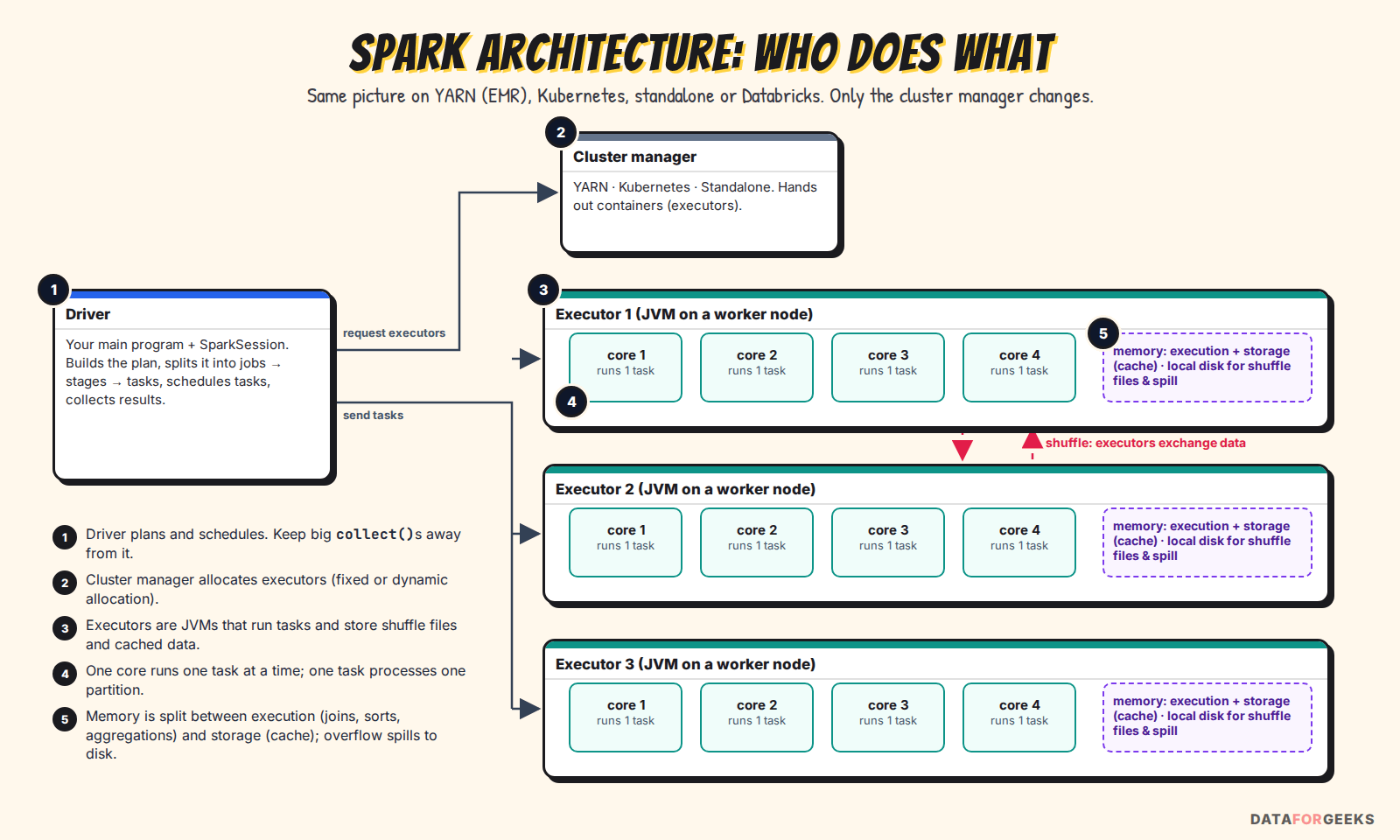
• Driver: runs your main program and the SparkSession. It turns your DataFrame code into a plan, splits it into jobs, stages and tasks, and schedules tasks on executors. It doesn’t process the bulk data itself, unless you ask it to with collect() or toPandas().
• Cluster manager: YARN on EMR, Kubernetes, Spark standalone, or Databricks’ own. It hands out containers; it knows nothing about your query.
• Executors: JVM processes on worker nodes. Each has a number of cores (task slots) and some memory. They run tasks, keep cached data, and write shuffle files to local disk.

The rule that matters most for this question: one task slot runs one task at a time, and one task processes one partition. By default a slot is one core (slots per executor = spark.executor.cores ÷ spark.task.cpus). So your parallelism is min(number of partitions, total task slots), and a single oversized partition is processed by a single slot, one core, no matter how big the cluster is.

Application, jobs, stages and tasks

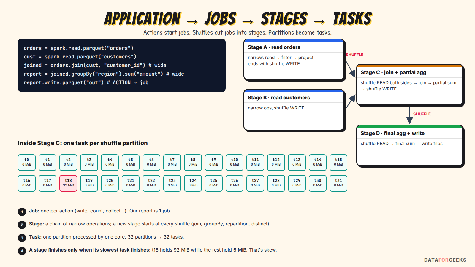
Level	Created by	In our demo
Application	One SparkSession / spark-submit	slow-job-demo
Job	Each action: write, count, collect, show… Some actions add extra jobs: sampling for orderBy, schema inference, collecting a broadcast table, and AQE, which runs stages as separate jobs	The report write = 1 job without AQE; 4 jobs with AQE on
Stage	A chain of narrow operations; a new stage starts at every shuffle	Read orders · read customers · join + partial aggregate · final aggregate
Task	One per partition in the stage	32 shuffle partitions → 32 tasks in the join stage

Spark is lazy: join and groupBy only build a plan. Nothing runs until an action, which is why a “slow line of code” in your notebook is almost always the action at the end, not the line that looks expensive.

Narrow vs wide transformations (and why shuffles matter)

	Narrow	Wide (shuffle)
Examples	select, filter, withColumn, map, union	join (non-broadcast), groupBy, distinct, repartition, orderBy, window functions
Data movement	None: each output partition depends on one input partition	Rows move across the network so that equal keys meet in the same partition
Cost	Cheap, pipelined inside one stage	Write to local disk, send over the network, read, often sort
Where skew bites	Rarely	Here. All rows with the same key land in the same partition

What a shuffle actually does

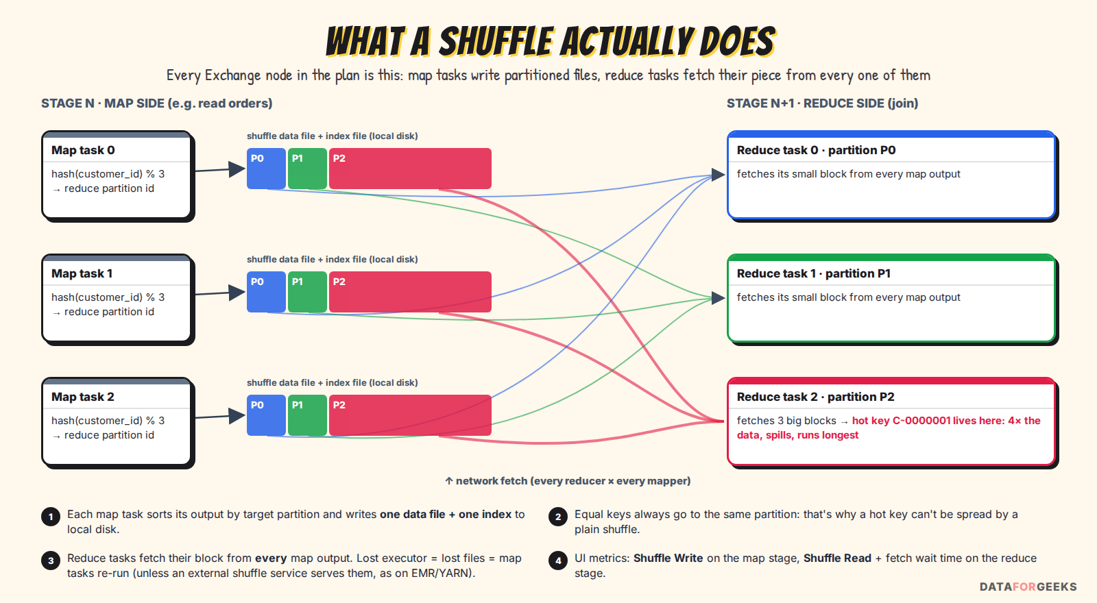
Every Exchange node in a query plan is a shuffle, and it’s the most expensive thing Spark does:

1. Map side: each task of the earlier stage computes hash(key) % numPartitions for every row, sorts its output by target partition, and writes one data file plus an index file to local disk. The UI shows this as Shuffle Write.
2. Reduce side: each task of the next stage fetches its block from every map output over the network (Shuffle Read, plus fetch wait time).
3. Failure behaviour: if an executor dies, its shuffle files die with it and the map tasks that wrote them must re-run, unless an external shuffle service keeps serving them (standard on YARN/EMR with dynamic allocation). Lost Spot nodes during a run therefore show up as re-run stages.

Which brings us back to the last row of the narrow-vs-wide table, the whole story of this post: a shuffle sends every row with key C-0000001 to the same partition, because it hashes the key. If that key owns 45% of the rows, one task gets 45% of the work.

From code to plan: Catalyst and AQE

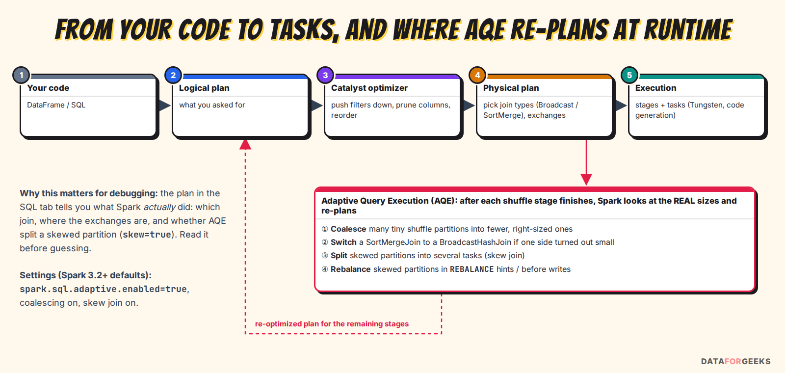
Spark’s Catalyst optimizer rewrites your query (pushing filters down, pruning columns) and picks a physical plan, including the join strategy. By default it broadcasts a table estimated below spark.sql.autoBroadcastJoinThreshold (10 MB) and otherwise uses a sort-merge join, which shuffles and sorts both sides.

The join strategies you’ll meet in plans:

Strategy	When Spark picks it	Shuffle?
Broadcast hash join	One side estimated under the broadcast threshold (10 MB), or a broadcast hint	No, for the big side
Sort-merge join	Default for large equi-joins (spark.sql.join.preferSortMergeJoin=true)	Both sides, plus a sort
Shuffled hash join	When sort-merge isn’t preferred, or AQE converts to it at runtime; the build side per partition must fit in memory	Both sides, no sort
Broadcast nested loop join / cartesian product	Non-equi joins (<, between, OR conditions); cartesian product if neither side can be broadcast	Compares every pair of rows: a classic hidden trap

Adaptive Query Execution (AQE), enabled by default since Spark 3.2, goes further: after each shuffle stage finishes it looks at the real partition sizes and re-plans the rest of the query. It can:

• merge small shuffle partitions (coalescing);
• switch a sort-merge join to a broadcast join (spark.sql.adaptive.autoBroadcastJoinThreshold), reading the already-written shuffle files locally with a local shuffle reader;
• switch a sort-merge join to a shuffled hash join when partitions are small enough (spark.sql.adaptive.maxShuffledHashJoinLocalMapThreshold, which is 0, i.e. off, by default);
• split skewed partitions in joins, and in REBALANCE hints.

The WholeStageCodegen (n) boxes you’ll see in the UI are Tungsten at work: Spark fuses a chain of operators into one generated Java function. A stage can contain several such blocks (our join stage has three), and the operators inside one block share a single duration metric.

Partitions: the unit of parallelism

Where	What decides the number	Default / rule of thumb
Reading files	spark.sql.files.maxPartitionBytes, file sizes and count	128 MB per partition; many tiny files = many tiny tasks
After a shuffle	spark.sql.shuffle.partitions, or AQE coalescing	200 by default; AQE targets advisoryPartitionSizeInBytes (64 MB)
Writing	Partitions of the final DataFrame, repartition / coalesce	Aim for files of roughly 128 MB–1 GB

A healthy stage has tasks of similar size, big enough to amortise overhead (tens to hundreds of MB), and at least as many tasks as cores. For the full list of knobs, see our Apache Spark performance tuning and best practices guide. This post focuses on how to diagnose which knob matters.

Executor memory and spill

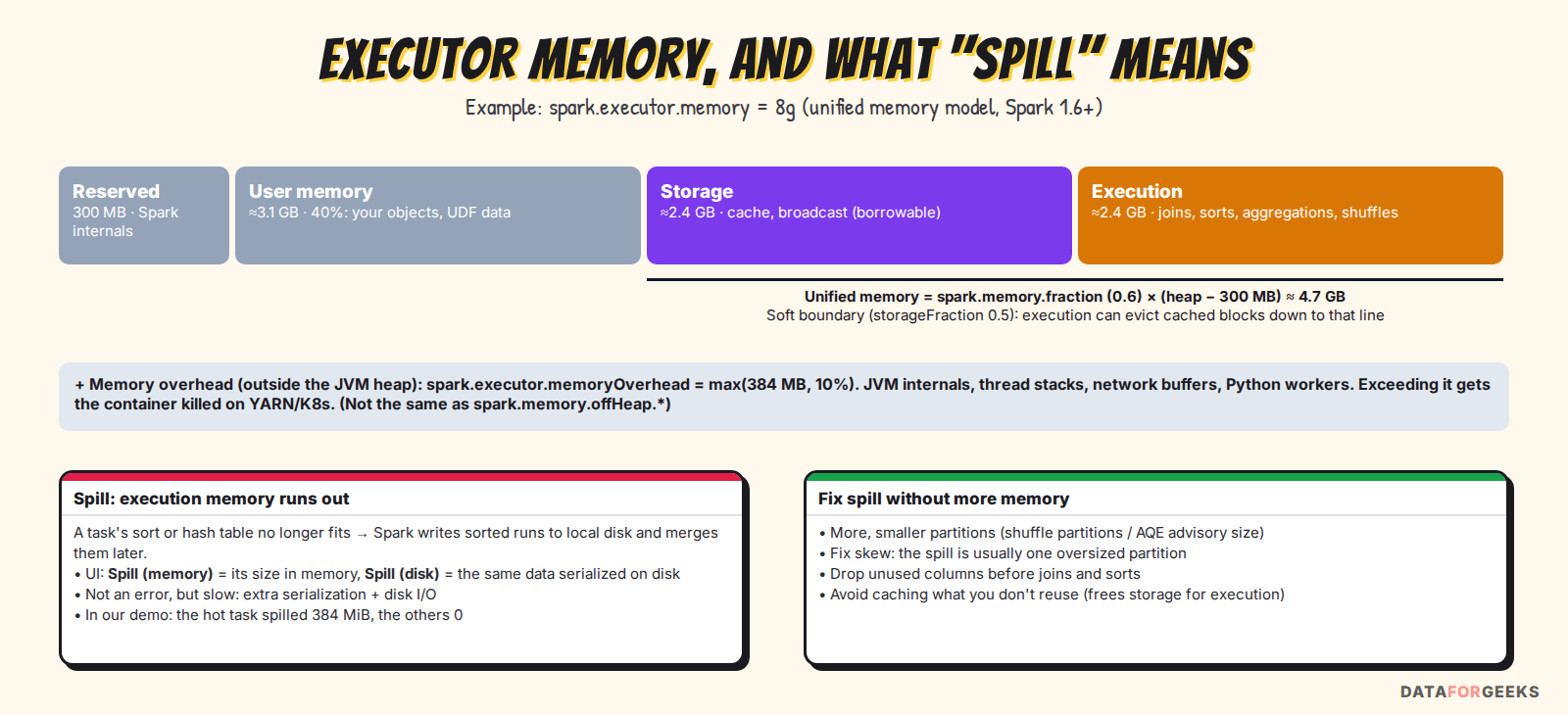
Joins, sorts and aggregations use execution memory. When one task’s sort buffer or hash table doesn’t fit, Spark doesn’t crash; it spills: writes sorted runs to local disk and merges them later. Spill is not an error, but it adds serialisation and disk I/O. When spill shows up in only one task, it’s almost always because that task’s partition is far bigger than the rest. Remember that pattern; the UI will show it to us in a minute.

For PySpark, Python worker memory comes out of the container’s overhead unless you set spark.executor.pyspark.memory; containers killed by YARN or Kubernetes for “exceeding memory limits” are usually an overhead problem, not a heap problem.

The demo: yesterday vs today, reproduced

To make the screenshots real, we reproduced the incident on a small scale with PySpark 4.0 on a laptop. The “daily report” joins orders to customers and aggregates revenue by region and segment:

def report(orders, customers):
    return (orders.join(customers, "customer_id")
                  .groupBy("region", "segment")
                  .agg(F.count("*").alias("orders"), F.sum("amount").alias("gmv")))

spark.sparkContext.setJobDescription("2 · Today: 24M orders, 45% one customer (SKEW)")
report(today, customers).write.format("noop").mode("overwrite").save()

• Yesterday: 8M orders spread evenly over 200,000 customers.
• Today: 24M orders (3× growth), and 45% of them belong to one customer, C-0000001. In real life this is a marketplace’s “guest checkout” account, a default ID from a buggy upstream release, or one enterprise client onboarding overnight.
• To mimic a legacy job, AQE and automatic broadcast are switched off, and shuffle partitions are set to 32.

Run	Data	Query time
Yesterday	8M orders, no skew	19 s
Today (the incident)	24M orders, 45% one customer	31 s
Control	24M orders, no skew	30 s
Fix A: AQE skew join	Today’s data	27 s
Fix B: salting (N = 16)	Today’s data	26 s
Fix C: broadcast join	Today’s data	15 s
Recommended: AQE + broadcast	Today’s data	13 s

Why the laptop hides the skew (and why that’s a lesson)

Look at “Today” vs “Control”: 31 s vs 30 s. If you only looked at wall-clock time, you’d blame volume and move on. That’s exactly the trap.

The reason is one formula worth memorising:

stage time ≈ max( slowest task , total task time ÷ task slots )

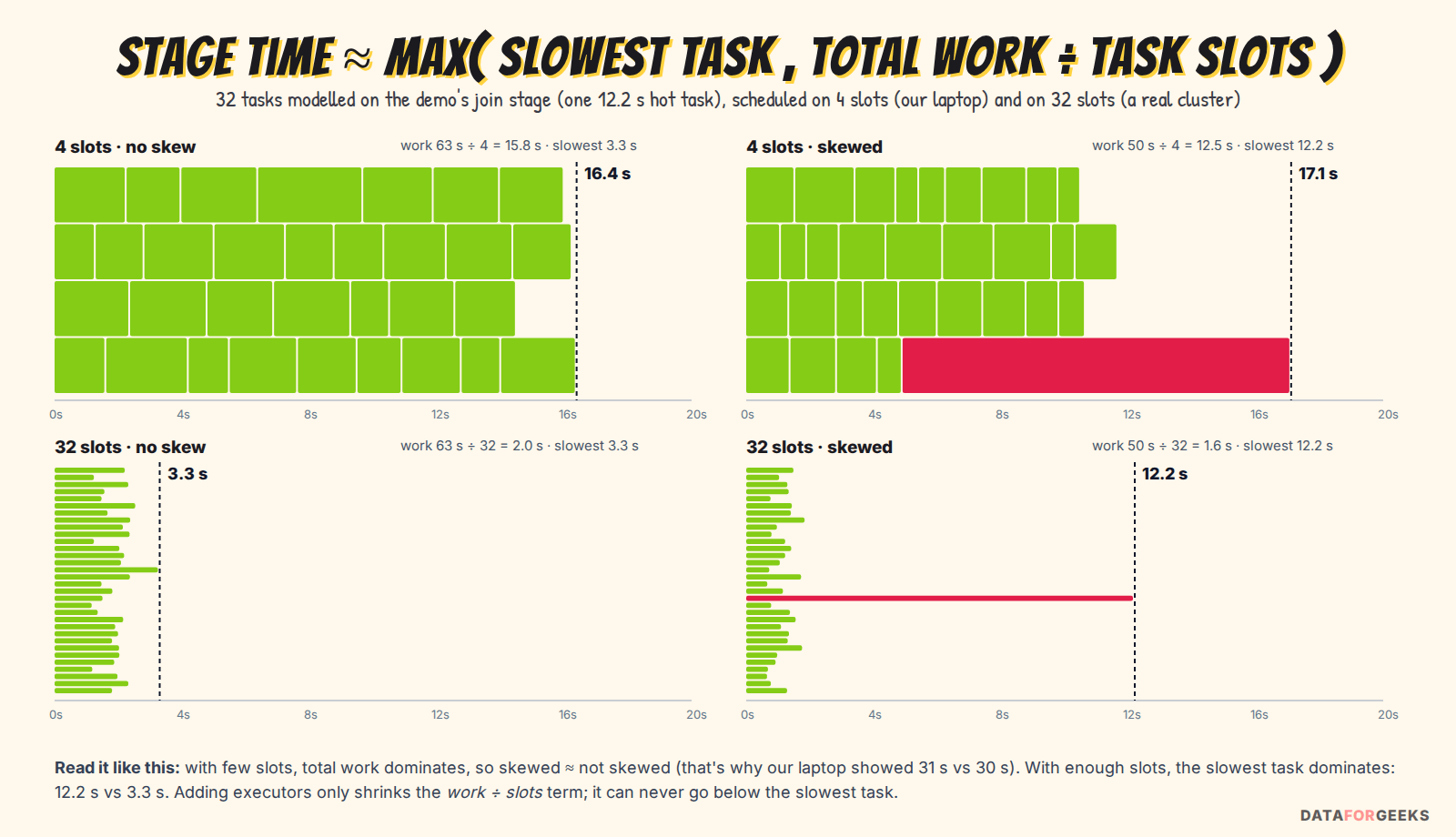
Our demo machine has only 4 task slots (on 2 CPU cores). The join stage’s 32 tasks run in about 8 waves, the second term of the formula dominates, and the skewed and even runs take about the same time. On a real cluster with 32+ slots, all tasks run at once, the first term takes over, and the stage takes as long as its slowest task: about 12 s skewed vs about 3 s without skew. That’s a 4× difference in the join stage from the same data volume. Scale that up to production data and you get 10 minutes → 45 minutes.

The same formula answers “why not add executors?”: more slots only shrink the second term. They can never push the stage below its slowest task.

The lesson Nikhil says out loud: wall-clock time tells you that something is slow; task-level metrics tell you why. So let’s open the UI.

How to read the Spark UI, tab by tab

The Spark UI runs on the driver (port 4040 while the application is alive) and in the Spark History Server afterwards. Nikhil walks it top-down: query → job → stage → task → plan, asking one question per screen and stopping as soon as he can name the cause.

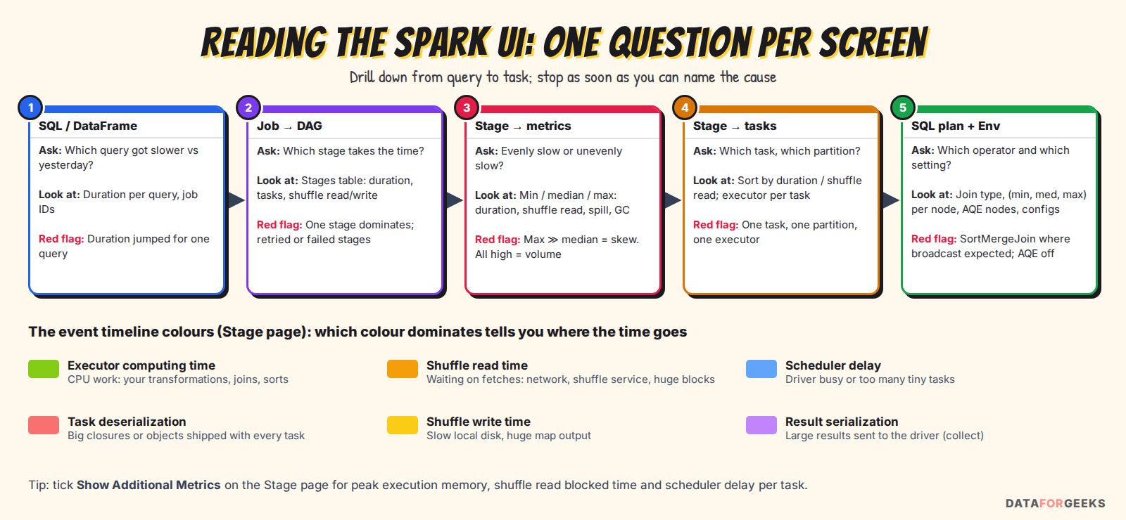
Tab	The question it answers
SQL / DataFrame	Which query got slower? What plan did it actually run?
Jobs	Which stages make up that query, and which one takes the time?
Stages	Inside the slow stage: are tasks evenly slow, or is one task the problem?
Executors	Are resources healthy? GC, failed tasks, lost executors, one bad node?
Environment	Which settings did this run really use?
Storage	What’s cached, and is it taking memory the job needs?

SQL / DataFrame tab: which query got slower

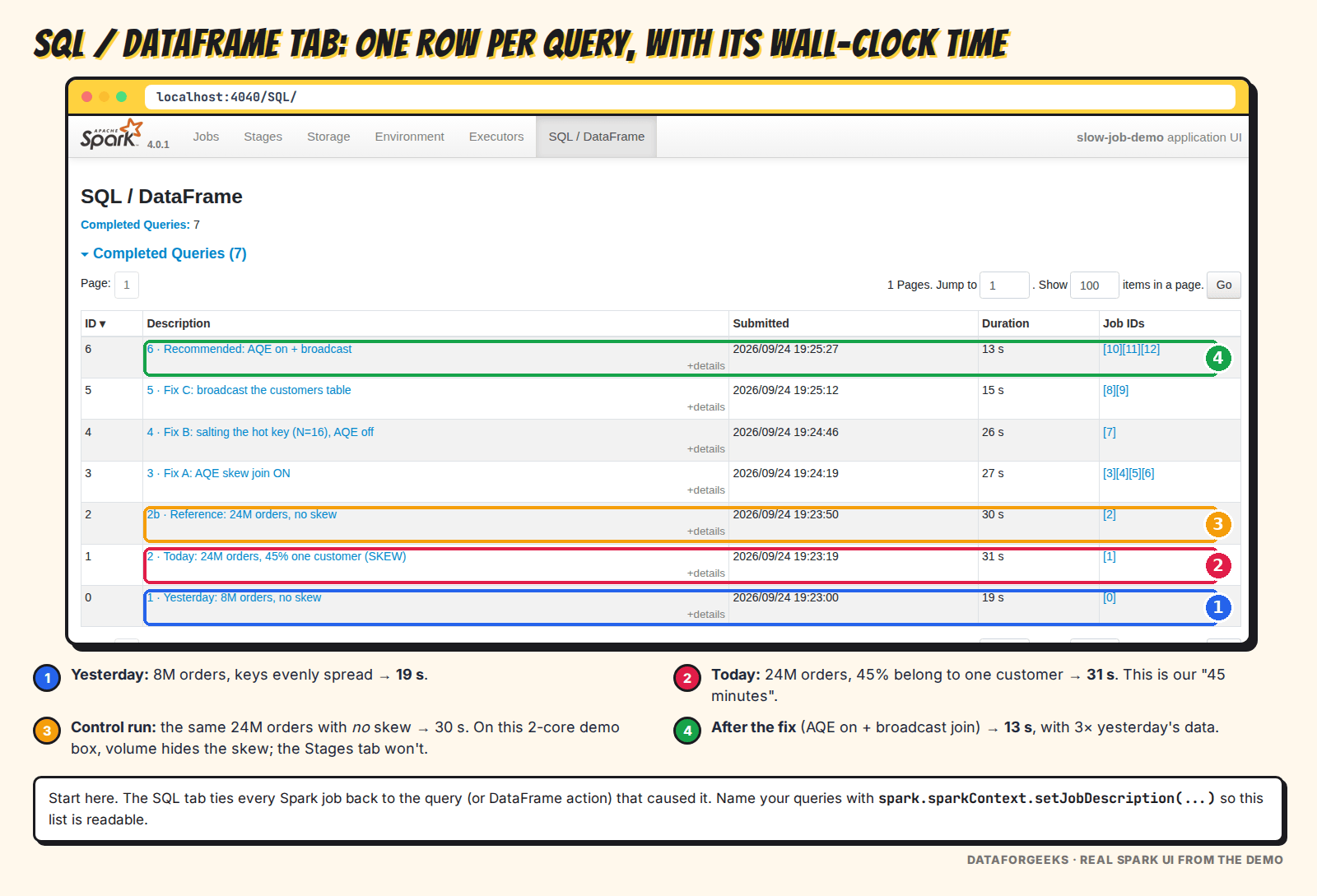
Each row is one query with its duration and the job IDs it triggered. In a real pipeline with dozens of steps, this is where you find the one step that grew. Naming steps with setJobDescription() (or spark.sql query comments) makes this page readable at 9 a.m.

Jobs tab: the DAG and the slow stage

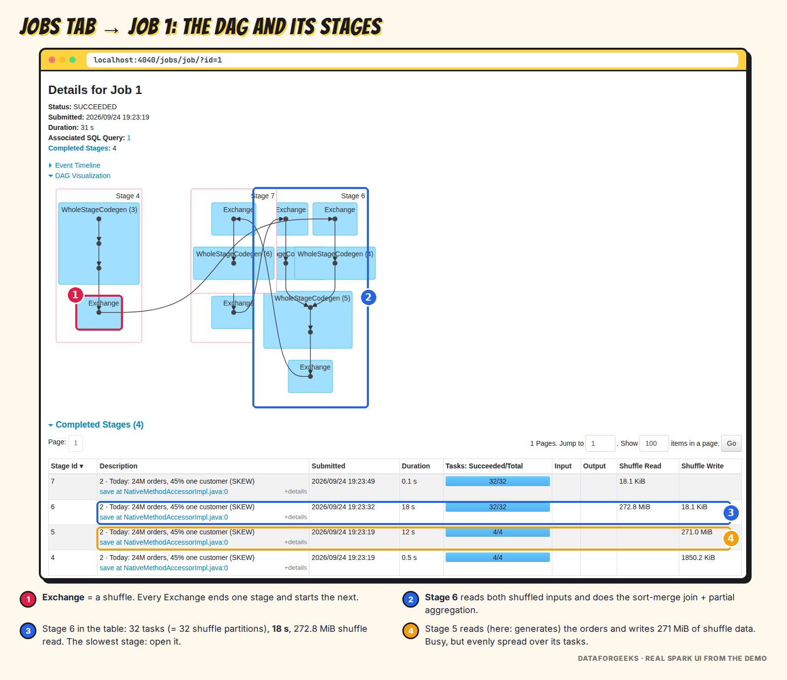
The DAG shows the stages and the Exchange (shuffle) nodes between them. The stages table below it is where you spot the offender: stage 6, the join, with 32 tasks and 18 s. Click it.

Two more things to check on this page: skipped stages (normal: output reused from an earlier job) and retried stages or failed tasks (not normal: fetch failures or lost executors, for example Spot reclaims, forcing recomputation). “It got slower today” is sometimes simply “it ran part of the job twice today”.

Stages tab: task quantiles tell the truth

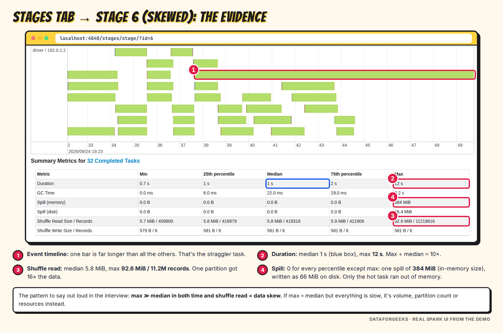
This is the most important screen in the whole investigation. The Summary Metrics table shows min, 25th percentile, median, 75th percentile and max for every task metric. Read it as a comparison between the median and the max columns:

• Duration: median 1 s, max 12 s.
• Shuffle read: median 5.8 MiB, max 92.6 MiB and 11.2M records.
• Spill: zero at every percentile except the max.

A note on reading spill, because it’s often misread: Spill (memory) is the size the spilled data had in memory, and Spill (disk) is the size of the same data once serialised and compressed on disk. So 384 MiB / 66 MiB is one spill, not two.

Also glance at the colours in the event timeline. Mostly green (computing) means CPU work, as here. Mostly orange (shuffle read) points to fetch or network problems. Lots of blue (scheduler delay) means a busy driver or too many tiny tasks. The reading map above lists them all.

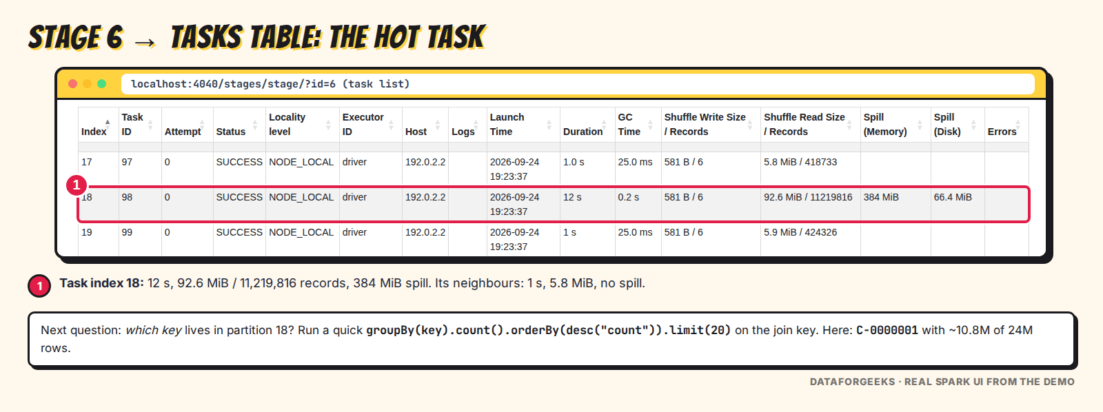
One task got 16× the data of a typical task, ran 10× longer, and was the only one to spill. That’s data skew, and you can now say it with evidence. The task list confirms which task it is:

Compare it with the control run: same 24M rows, no hot key. The quantiles are close together, the timeline is a neat brick wall, and nothing spills.

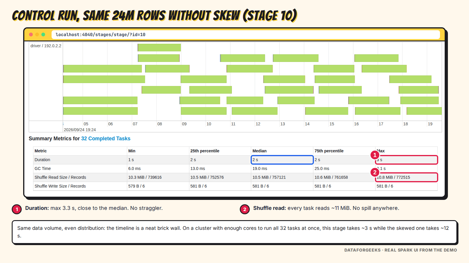
Join stage metric	Skewed (today)	No skew (control)
Task duration: median / max	1.2 s / 12.2 s	1.7 s / 3.3 s
Shuffle read: median / max	5.8 MiB / 92.6 MiB	~11 MiB / ~11 MiB
Spill	384 MiB (one task)	0
Stage time if all 32 tasks run at once	≈ 12 s	≈ 3 s

SQL plan: which operator suffered

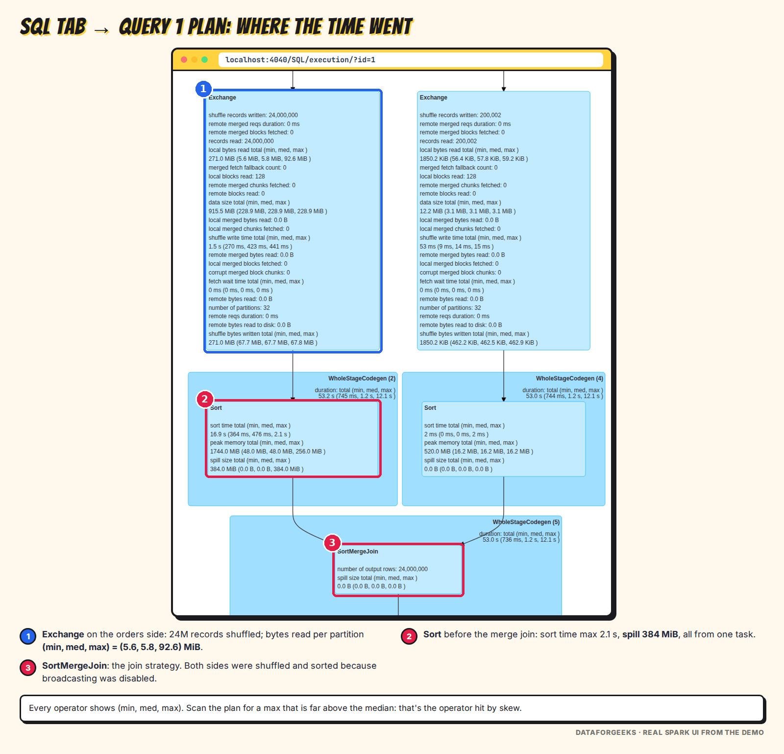
Click the query in the SQL tab to see the physical plan with runtime metrics on every node. Each metric is shown as total (min, med, max). Here the Exchange read (5.6, 5.8, 92.6) MiB per partition, the Sort in front of the join spilled 384 MiB from one task, and the join itself is a SortMergeJoin, even though one side is a small customers table. That last detail is a clue we’ll use in the fixes.

Environment and Executors tabs: settings and health

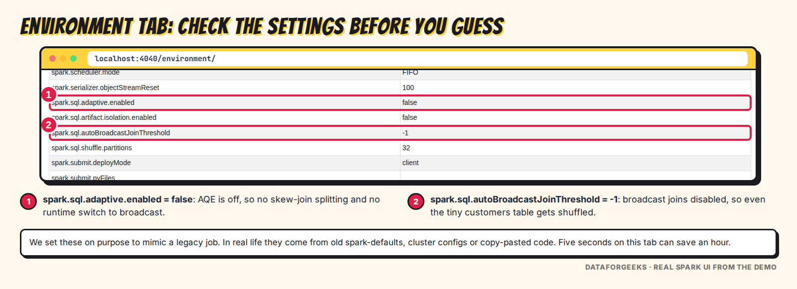
Before guessing, check what the run actually used. Here AQE is off and broadcast joins are disabled. In real incidents these come from old spark-defaults.conf files, cluster-level configs or a copy-pasted --conf, and a config that was harmless on even data becomes expensive when the data changes shape.

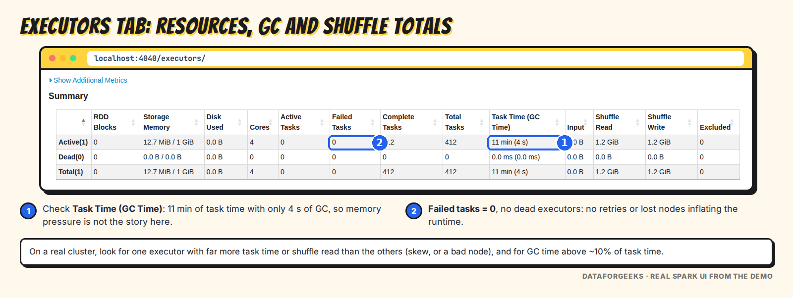
The Executors tab rules out the other usual suspects: GC time is tiny (4 s of 11 min), no failed tasks, no dead executors. On a multi-node cluster, also look for one executor with far more task time or shuffle read than the others (skew again, or a bad node).

Where to find the Spark UI on EMR, EMR Serverless and Databricks

Platform	Running job	Finished job
Amazon EMR on EC2	Cluster → Applications → Spark UI (or YARN ResourceManager → ApplicationMaster)	Persistent application UI / Spark History Server from the EMR console, backed by event logs
EMR Serverless	Job run → Spark UI	Job run → Spark History Server
Databricks	Compute → your cluster → Spark UI, or the job run’s Spark UI link	Same links, while the logs are retained; serverless SQL uses the query profile instead
Self-managed / Kubernetes	Driver port 4040 (port-forward on K8s)	Spark History Server with spark.eventLog.enabled=true and a shared log directory (S3 / HDFS)

The UI is the same everywhere; only the door is different. On EMR, also check the step’s stderr and YARN container logs if tasks failed, and whether Spot instances were reclaimed during the run: lost executors mean recomputed stages.

Data skew in Spark: detect it and fix it

What is data skew in Spark, and why more executors don’t help

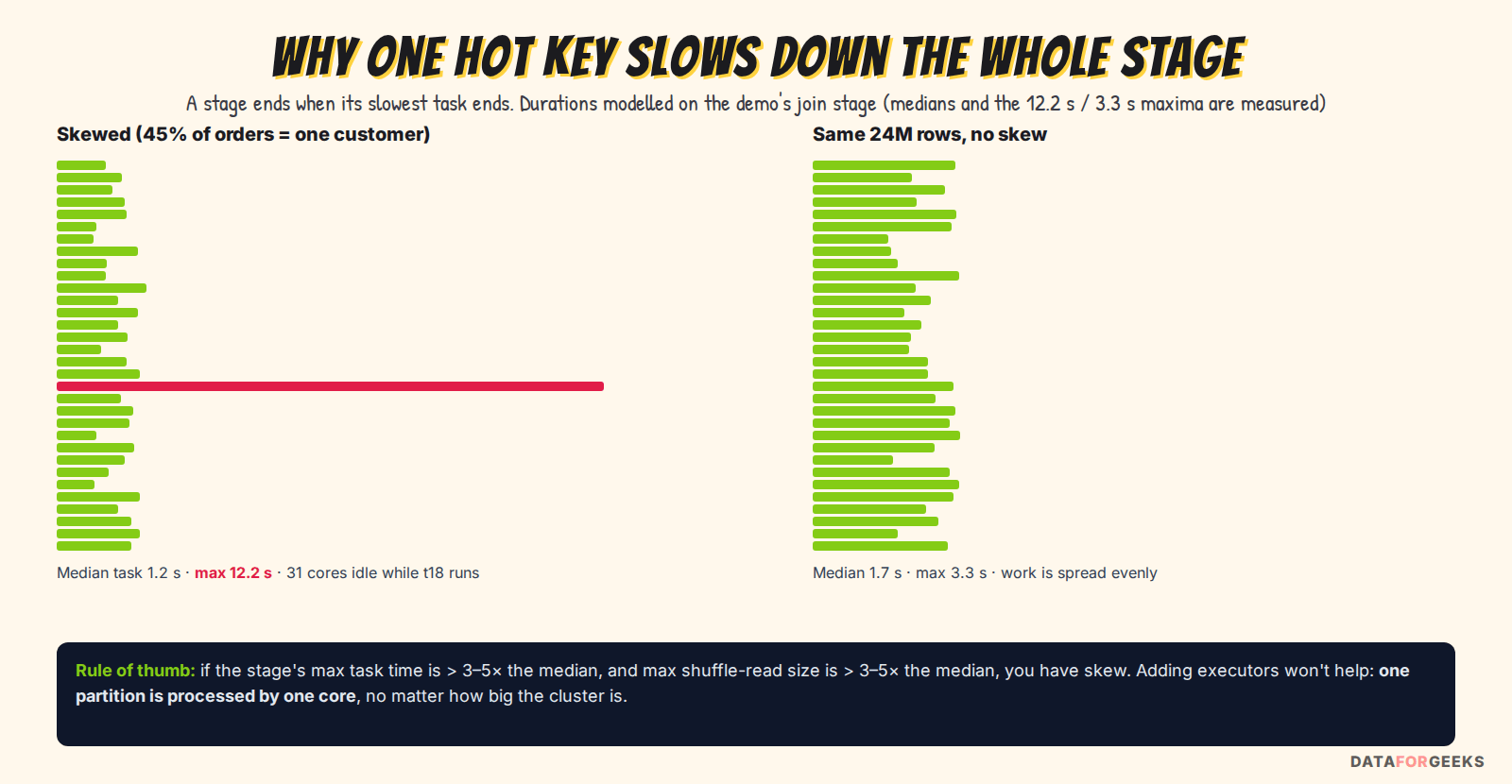
Data skew in Spark means data is unevenly spread across partitions, so a few tasks do most of the work. Since a stage ends when its last task ends, the whole cluster waits for that one core. Doubling the cluster would halve the time of the 31 small tasks, which were never the problem, and leave the 12-second task exactly as slow.

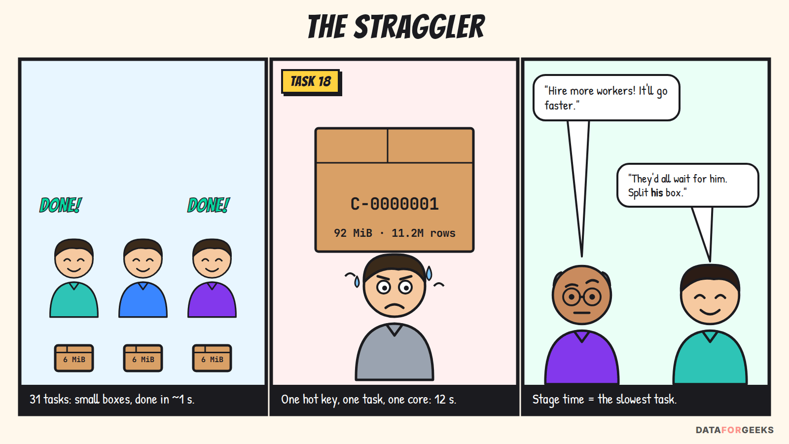
Skew mostly appears after a shuffle, because hash partitioning sends every row with the same key to the same partition. The usual victims:

• Joins on a key with a few very frequent values (the most common case, and ours).
• Aggregations (groupBy) on such a key, especially non-combinable ones like collect_list.
• Window functions partitioned by such a key.
• Writes partitioned by a column where one value dominates.
• Input files of very different sizes (one 5 GB gzip file can’t be split and becomes one task).

How to detect data skew

In the UI, three signals together:

1. Stage summary metrics: max duration ≫ median (a common rule of thumb is more than 3–5×).
2. Max shuffle read ≫ median, in bytes and records.
3. Spill and GC concentrated in the max column, and a long straggler bar in the event timeline.

Then confirm it in the data and find the culprit keys:

# 1. Which keys are hot? (sample first on huge tables)
(orders.groupBy("customer_id").count()
       .orderBy(F.desc("count")).limit(20).show())

# 2. How uneven are the partitions right now?
(orders.repartition(32, "customer_id")
       .groupBy(F.spark_partition_id().alias("pid")).count()
       .orderBy(F.desc("count")).show(5))

# 3. Watch for junk keys
orders.select(F.count(F.when(F.col("customer_id").isNull(), 1)).alias("null_keys")).show()

In the demo, the first query returns C-0000001 with about 10.8M of 24M rows. The next question is a business one, and a good candidate asks it: is this key real?

These checks also tell you which kind of skew you have, and that decides the fix:

• Single-key skew: one key owns the big partition. More shuffle partitions can’t help, because the key still hashes to one partition. You need AQE splitting, broadcast, isolation or salting.
• Hash-collision skew: several medium-sized keys happen to hash to the same partition. Here more partitions (or AQE’s sizing) does help, because they spread out.

Where skew comes from

Cause	Example	Best first move
Junk or default keys	NULL, '', 'unknown', -1, 0, test accounts	Filter or handle separately; fix upstream
Real-world power law	A marketplace’s biggest seller, a viral product, a huge enterprise tenant	Broadcast, AQE skew join, isolate hot keys, salting
Sudden new behaviour	A new client onboarded, a campaign, a bot	Same as above, and alert on key share
Upstream bug	A release writes the same ID into every row	Data quality check; stop the pipeline rather than “fix” it in Spark
Partition column choice	Writing partitionBy("country") when 70% is one country	Add a second key or salt when writing

Fix: turn on AQE skew join

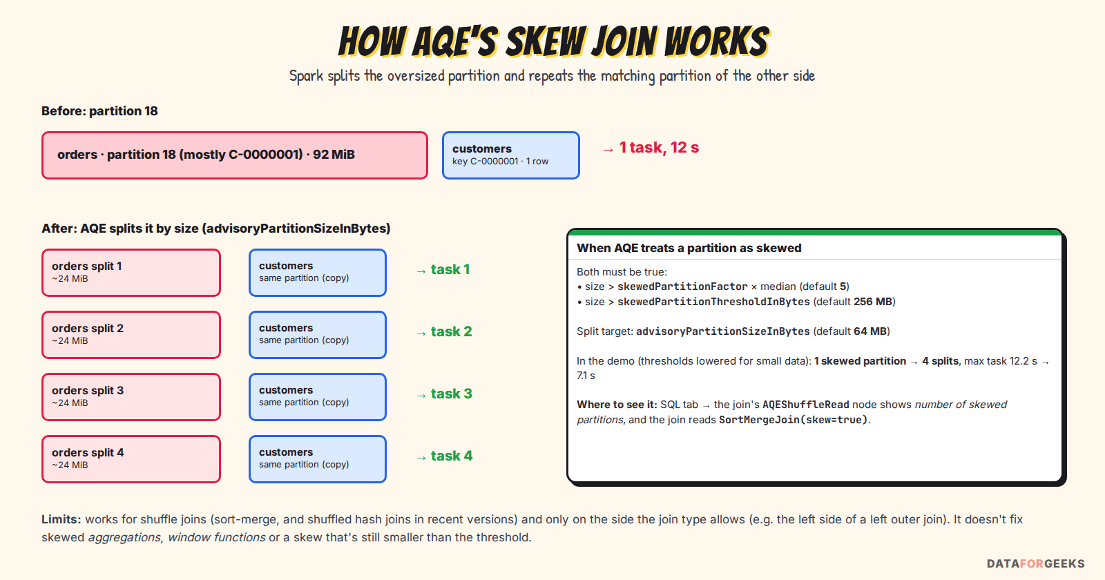
With AQE on, after the shuffle Spark knows every partition’s real size. A partition is treated as skewed when it is larger than both skewedPartitionFactor × the median partition size and skewedPartitionThresholdInBytes. Spark then splits it into chunks of about advisoryPartitionSizeInBytes, and joins each chunk with a copy of the matching partition from the other side.

spark.sql.adaptive.enabled=true                                   # default since 3.2
spark.sql.adaptive.skewJoin.enabled=true                          # default true
spark.sql.adaptive.skewJoin.skewedPartitionFactor=5               # default 5
spark.sql.adaptive.skewJoin.skewedPartitionThresholdInBytes=256MB # default 256MB
spark.sql.adaptive.advisoryPartitionSizeInBytes=64MB              # default 64MB

The demo’s data is tiny, so we lowered the thresholds (factor 3, 16 MB) to make AQE react. In production the defaults are usually right; lower them only if the UI shows a skewed partition that AQE ignored. You can check whether it worked in the plan:

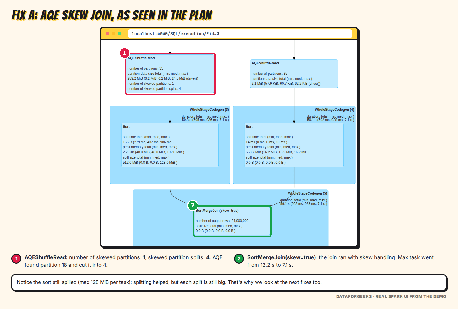
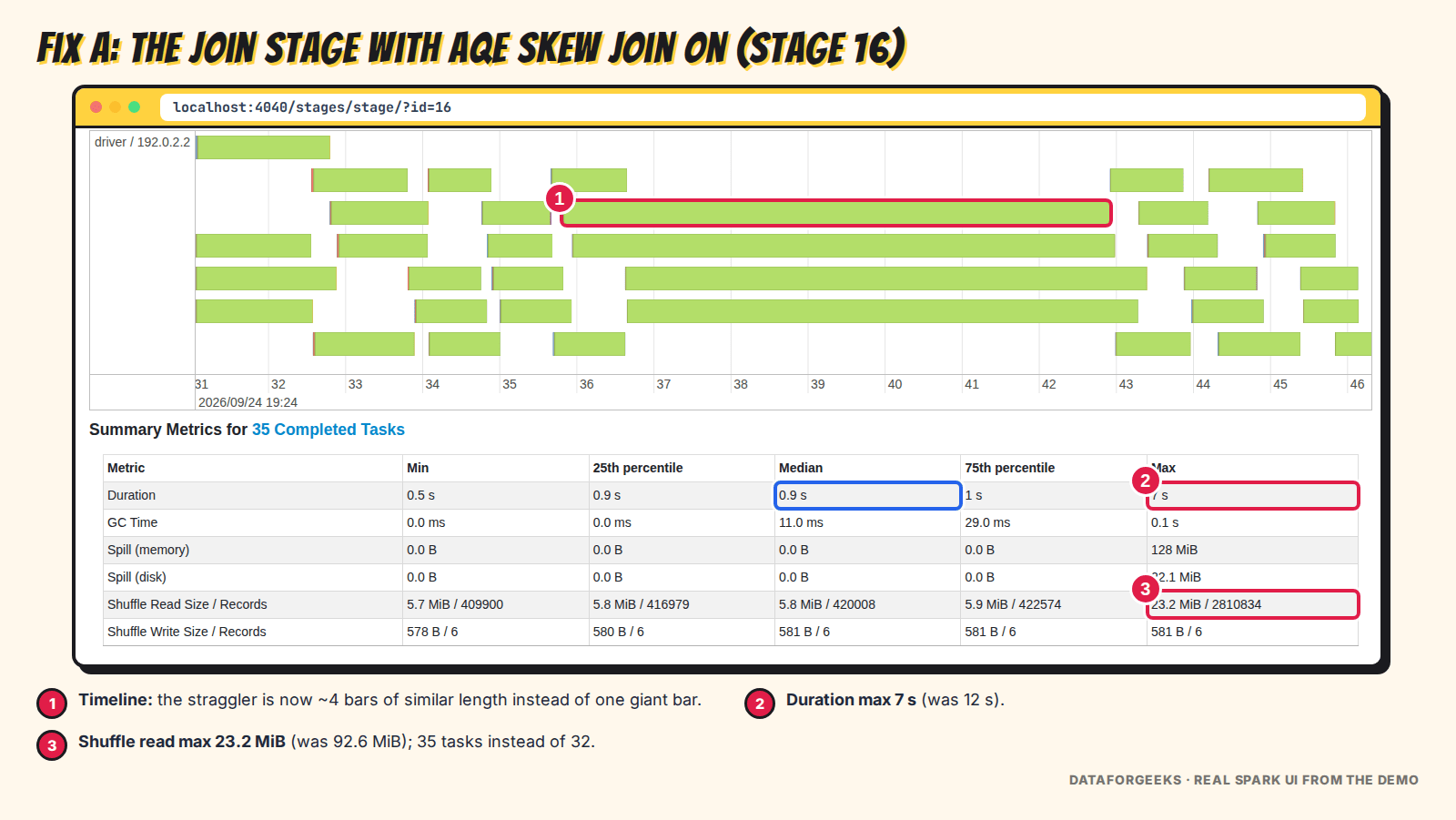
Result: max task 12.2 s → 7.1 s, max shuffle read 92.6 → 23.2 MiB, with zero code changes. It isn’t perfect, because each split still spills a little, but it’s the cheapest fix available.

Where AQE skew join doesn’t help:

• It only handles shuffle joins (sort-merge; shuffled hash join in newer versions). It doesn’t touch skewed groupBy, window functions or writes.
• It can only split the side the join type allows, for example the left side of a left outer join. Check your Spark version’s docs for full outer joins.
• It skips a split that would need an extra shuffle (unless spark.sql.adaptive.forceOptimizeSkewedJoin is set, Spark 3.3+), and it ignores skew below the thresholds.

Fix: broadcast the small side

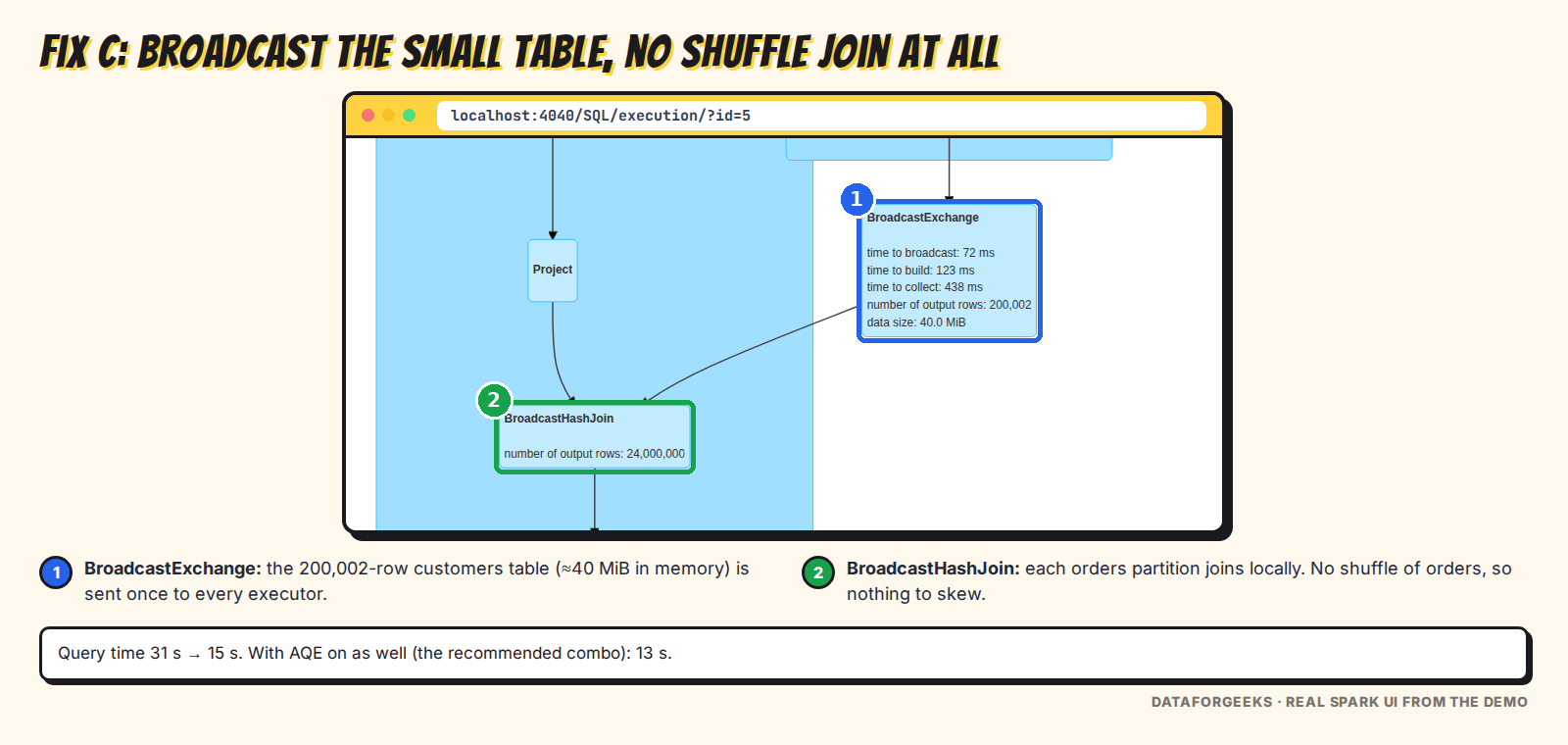
If one side of the join is small, don’t shuffle the big side at all. A broadcast hash join sends the small table once to every executor, and each partition of the big table joins locally. No shuffle of orders means no hot partition, so skew simply disappears.

from pyspark.sql import functions as F
report = orders.join(F.broadcast(customers), "customer_id")   # explicit hint

# or let Spark decide by size (default 10MB, estimated size)
spark.conf.set("spark.sql.autoBroadcastJoinThreshold", "64MB")

Result: query time 31 s → 15 s (13 s with AQE also on). This is also a classic answer to the “since yesterday” puzzle: if the small table grows past 10 MB (or its estimated size does), Spark silently switches from a broadcast join to a sort-merge join, and a job that never shuffled its big table suddenly does.

Why “small” is tricky: for file sources, Spark estimates size from the on-disk, compressed files, while the broadcast is built from decoded rows. Our customers table is about 40 MiB in memory; a 5 MB Parquet file can easily be 50 MB once decoded. Estimates after filters and joins can be even further off. AQE’s runtime switch uses real shuffle sizes, which is one more reason to keep it on.

Limits: the table must fit in the driver’s and every executor’s memory (hard limit 8 GB, but in practice keep it to tens or a few hundred MB); it’s built on the driver first; and in outer joins only the non-preserved side can be broadcast (the right side of a left join; never a full outer join). A too-large broadcast is itself a common cause of driver OOMs and broadcast timeouts.

Fix: salt the hot key

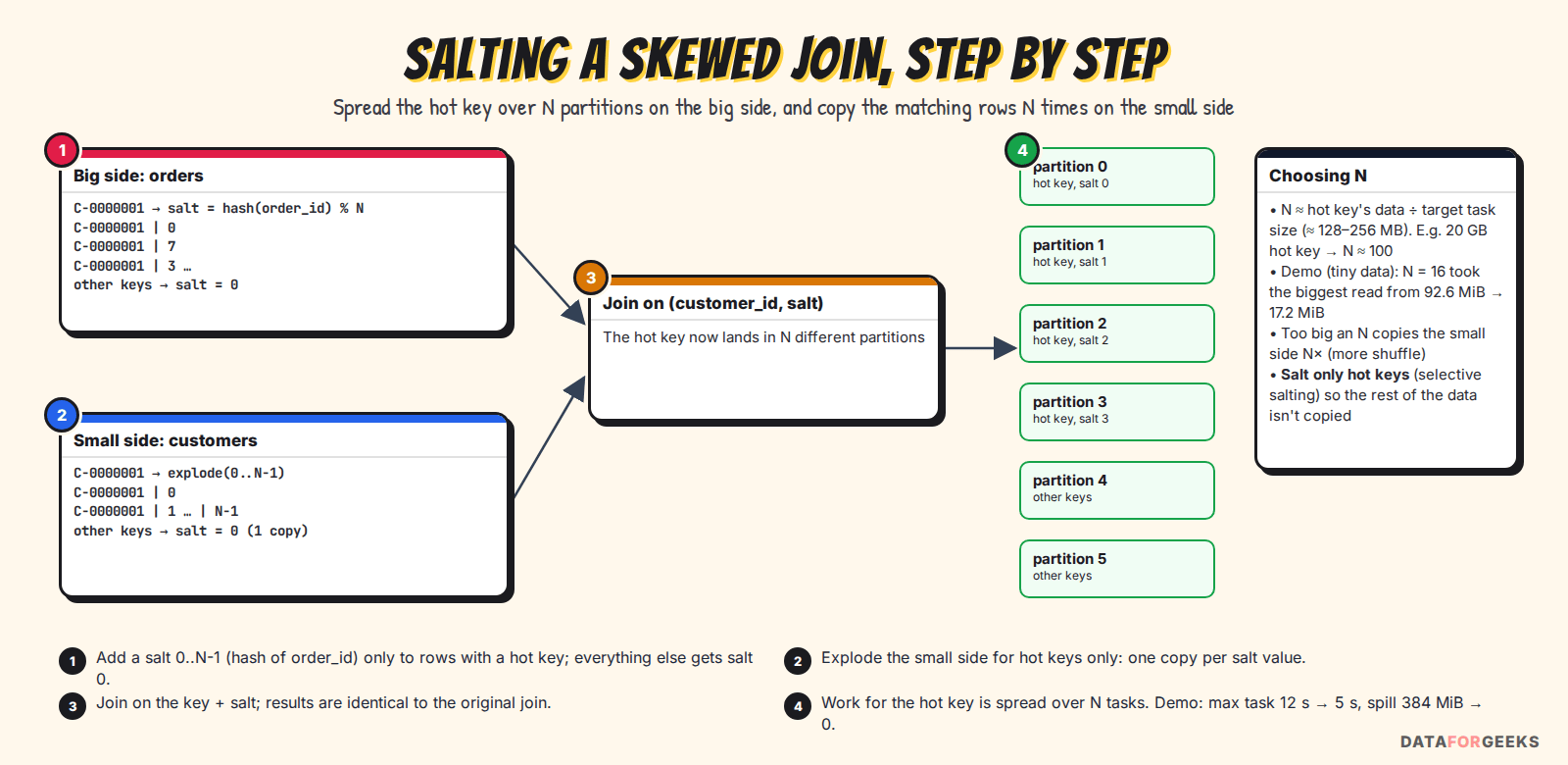
When both sides are big, broadcast isn’t possible. Salting spreads the hot key over N partitions: add a salt value 0..N-1 to the hot key’s rows on the big side, copy the matching rows N times on the other side, and join on (key, salt). The result is identical; the work is spread out.

N   = 16
hot = ["C-0000001"]            # from the top-keys query, or a daily job that finds them

# deterministic salt from a unique column (safer than rand() if a stage is retried)
orders_s = orders.withColumn(
    "salt",
    F.when(F.col("customer_id").isin(hot), F.pmod(F.xxhash64("order_id"), F.lit(N)))
     .otherwise(F.lit(0)))

customers_s = customers.withColumn(
    "salt",
    F.explode(F.when(F.col("customer_id").isin(hot),
                     F.array(*[F.lit(i) for i in range(N)]))
               .otherwise(F.array(F.lit(0)))))

joined = orders_s.join(customers_s, ["customer_id", "salt"]).drop("salt")

Why a hash of order_id instead of rand()? A random value computed before a shuffle makes that stage non-deterministic: if a fetch fails and Spark has to recompute some map output, rows could land in different partitions than the first time. Spark handles this by re-running the whole stage, which is slow; a deterministic salt avoids the problem. (Our demo used rand() for brevity.)

This is selective salting: only hot keys are salted, so only their few matching rows are copied. Salting every key would multiply the whole small side by N and add shuffle for nothing, which is a common mistake in interview answers.

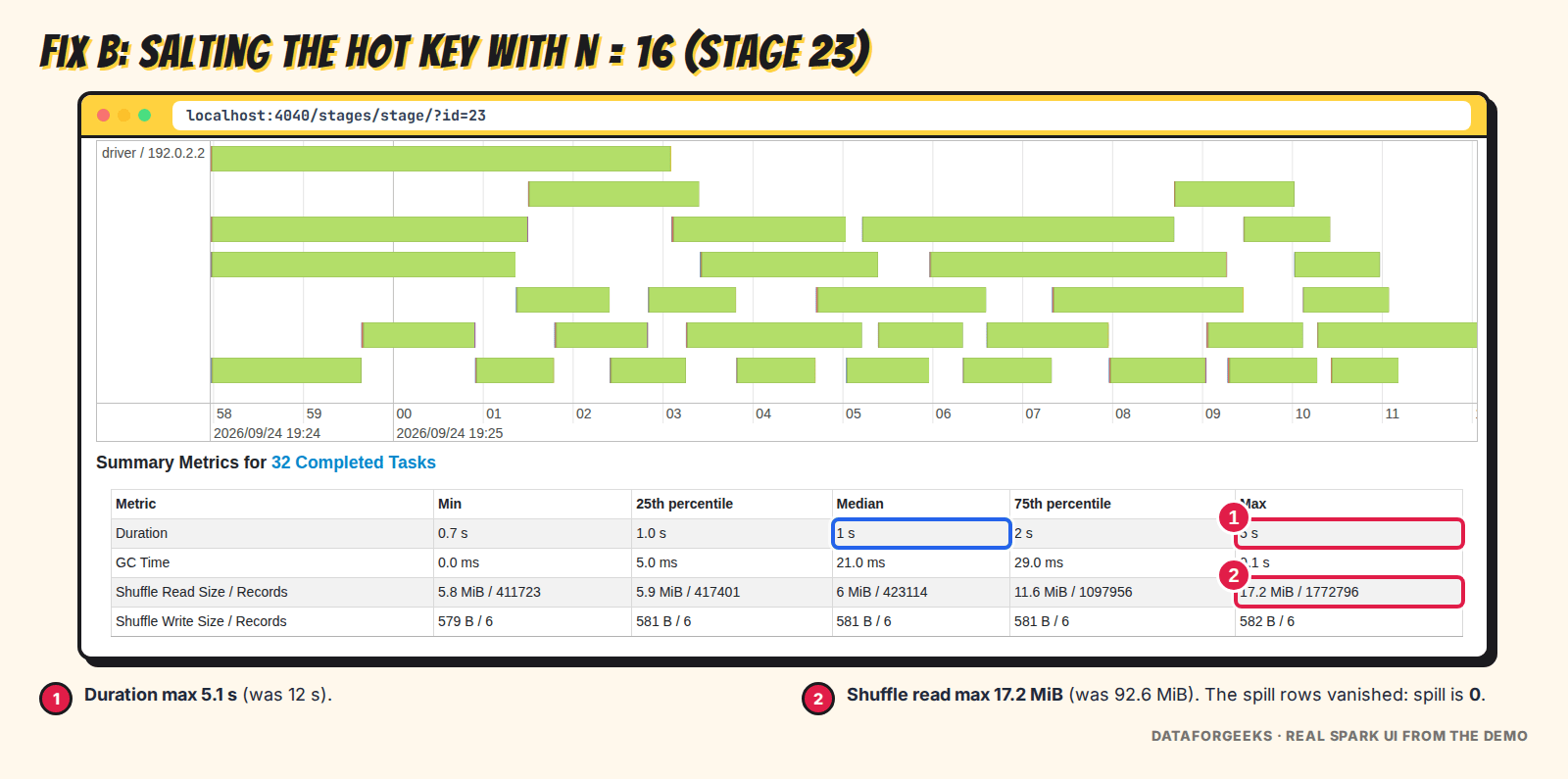
Result: max task 12.2 s → 5.1 s, max shuffle read 92.6 → 17.2 MiB, spill 384 MiB → 0. Choosing N: roughly the hot key’s data size divided by a healthy task size (128–256 MB). Too small and the hot key is still a straggler; too big and you copy the small side more than needed.

Fix: two-stage aggregation for a skewed groupBy

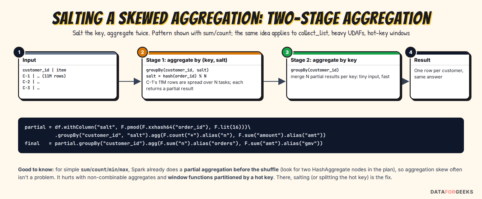
Good news first: for sum, count, min, max and avg, Spark already does a partial aggregation before the shuffle (you’ll see two HashAggregate nodes in the plan), so a hot key sends only one partial row per task. Aggregation skew hurts when the aggregate can’t be pre-combined cheaply, such as collect_list, exact percentiles or heavy UDAFs. Then aggregate twice: first by (key, salt), then by key. As with joins, prefer a deterministic salt (a hash of a unique column) over rand(). Also watch several countDistincts in one query: Spark expands each row once per distinct aggregate (an Expand node in the plan), which can multiply the shuffle several times over.

Fix: isolate the hot keys and union

When you know the few hot keys, process them on a separate path and union the results:

is_hot = F.col("customer_id").isin(hot)

normal = orders.filter(~is_hot).join(customers, "customer_id")              # regular shuffle join
hot_rows = orders.filter(is_hot).join(
    F.broadcast(customers.filter(F.col("customer_id").isin(hot))), "customer_id")  # tiny broadcast

joined = normal.unionByName(hot_rows)

This keeps the big path untouched and gives the hot rows a broadcast join against a handful of customer rows. It’s easy to explain and easy to debug, which matters at 2 a.m.

Fix: drop or route junk keys

If the hot key is NULL, an empty string or a placeholder like 'unknown', the best fix happens before the join.

• NULL keys in an inner join: Spark’s optimizer already adds an isnotnull(key) filter for inner equi-joins, so NULLs never reach the shuffle. If you see NULL skew, look for an outer join.
• NULL keys in an outer join: the rows must stay, and they all hash to one partition. Replace the NULL with a random value that can never match, so the rows spread out and still come back unmatched:

  orders.withColumn("join_key",
      F.coalesce(F.col("customer_id"),
                 F.concat(F.lit("__null_"), F.pmod(F.xxhash64("order_id"), F.lit(64)).cast("string"))))
  # join on join_key = customers.customer_id: the "__null_…" values never match,
  # so these rows stay unmatched (as before) but are spread over 64 partitions

• Placeholders ('', 'unknown', -1): Spark treats these as real values, so filter them or route them separately.
• Upstream bugs: if the “hot key” exists because of a bad release, the right answer is a data quality check that stops the pipeline, not a clever Spark trick.

Skew in window functions and writes

• Window functions: Window.partitionBy("customer_id") puts every row of the hot customer in one task. Salting only works if the calculation can be split and recombined (a running sum per day, then a sum of sums). For row_number() across the whole key, isolate the hot key or change the logic, for example compute per day first.
• Writes: partitionBy("date") with one huge date means one task writes a giant file. Use repartition("date", salt) or spark.sql.files.maxRecordsPerFile, or the REBALANCE hint, which AQE can split when it is skewed.
• Hints on Databricks: Databricks also accepts a SKEW hint, for example /*+ SKEW('orders', 'customer_id') */. It’s Databricks-specific, and with AQE it’s rarely needed; open-source Spark ignores it.

Choosing a fix

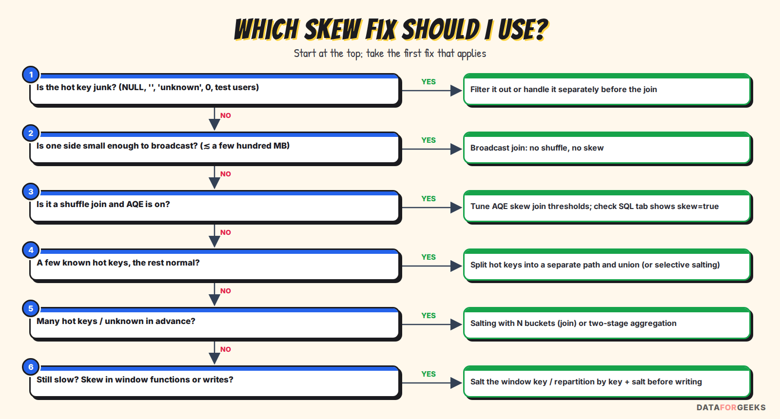
Fix	Effort	Works for	Watch out for
Filter / route junk keys	Low	NULL and placeholder keys	Don’t drop rows an outer join must keep
Broadcast join	Low	One side small	Driver/executor memory, outer-join side rules
AQE skew join	Config only	Shuffle joins	Thresholds; not for groupBy, windows or writes
Isolate hot keys + union	Medium	A few known hot keys	Keeping the hot-key list current
Salting	Medium	Big-big joins, unknown hot keys	Choosing N, copying the small side
Two-stage aggregation	Medium	Non-combinable aggregates	Only for aggregates that can be merged

Other causes of a slow Spark job

Skew is the classic answer, but a strong candidate shows they’d rule out the others. Same method: symptom → where you see it → fix, without spending more.

Suspect	What you see in the UI	Fix at the same cost
Broadcast join became sort-merge	Plan shows SortMergeJoin + new Exchange where yesterday had BroadcastHashJoin	Broadcast hint, sensible threshold, AQE (can switch at runtime)
Too few shuffle partitions for the new volume	Median task is big and slow, spill in most tasks	Raise spark.sql.shuffle.partitions or let AQE size them
Too many tiny partitions / files	Thousands of millisecond tasks, high scheduler delay, slow file listing	Compact files, AQE coalescing, maxPartitionBytes
Lost partition pruning / filter pushdown	Input size jumped; no PartitionFilters in the scan node	Filter directly on the partition column; don’t wrap it in functions
Join explosion from duplicates	Join output rows ≫ input rows	Deduplicate; add a uniqueness check upstream
Python UDF	BatchEvalPython / ArrowEvalPython nodes taking the time	Built-in functions, or vectorised pandas UDFs
Memory pressure / GC	GC time above ~10% of task time in the Executors tab	Smaller partitions, fewer cached objects, drop unused columns
Recomputation	The same stages run twice for one DataFrame used twice	persist() what’s reused, unpersist() after
A slow or sick node	One executor slow for all its tasks, whatever their size	spark.speculation (only with idempotent output), exclude the node
Fewer resources than usual	Fewer executors in the timeline, pending tasks, lost Spot nodes	Queue / scheduling, run window, retries: no hardware change needed
Executors that don’t fill the cluster	YARN / Executors tab: fewer cores in use than the nodes have (1-core executors, memory rounding that fits 2 executors where 3 would fit)	Right-size spark.executor.cores (often 4–5) and memory to the instance type: same nodes, more slots
Stage retries / fetch failures	Retried stages, FetchFailed errors, lost executors (Spot reclaims)	External shuffle service, Spot for task nodes only, fix the failing node
Non-splittable input	One input task reading a huge .gz / .zip file	Columnar formats (Parquet/ORC split by row group with any codec), bzip2 for text, or smaller files upstream
Many countDistincts	Expand node multiplying rows before the shuffle	approx_count_distinct, or compute distinct counts separately
Driver bottleneck	Long gaps between jobs, collect() / toPandas() on big data	Keep work distributed; write results out instead of collecting

For the tuning parameters behind these fixes (executor sizing, serialisation, caching, file formats), our Spark performance tuning guide goes knob by knob.

How to fix a slow Spark job without extra cost

Nikhil closes the loop with numbers from the demo. Same laptop, same data, nothing added:

Version	Query time	Join stage: max task	Max shuffle read	Spill	Change
Today (skewed)	31 s	12.2 s	92.6 MiB	384 MiB	–
Fix A: AQE skew join	27 s	7.1 s	23.2 MiB	128 MiB max per task	Config only
Fix B: selective salting	26 s	5.1 s	17.2 MiB	0	Code change
Fix C: broadcast customers	15 s	no shuffle join	–	0	One-line hint
AQE on + broadcast	13 s	no shuffle join	–	0	Config + hint

And the order he’d apply them in production:

1. Restore sane configs: AQE on, broadcast threshold not -1. Zero code, zero cost.
2. Broadcast the dimension table if it’s small; check its size trend so it doesn’t silently cross the limit later.
3. For big-big joins, check that AQE splits the skewed partitions; tune its thresholds only if the UI shows it didn’t.
4. If skew persists, isolate the known hot keys or salt selectively.
5. Fix the data: filter junk keys early and raise the upstream bug if the hot key shouldn’t exist.
6. Verify performance with the same metrics: stage max vs median, spill, total runtime vs yesterday.
7. Verify correctness: salting and hot-key splitting are code changes. Compare row counts and key totals (e.g. sum of gmv per region) between the old and new versions on the same input before switching.

Preventing Spark performance regressions

• Runtime alerts against a baseline: alert when a run exceeds, say, 1.5× the median of the last 14 runs, not a fixed number that’s wrong after every growth spurt.
• Input and key-distribution checks: row counts per day, null-key rate, and the share of the top key. “One customer owns 45% of today’s orders” should be a data quality alert before it’s a performance incident.
• Keep the evidence: event logs on durable storage (S3) and a History Server, so yesterday’s good run is always there to compare against.
• Config hygiene: job configs in version control and code review; no cluster-wide -1s left over from an old experiment.
• Stage-level metrics: export task duration and shuffle-read quantiles per stage (Spark listeners, the REST API or your platform’s metrics) and alert on max ÷ median.
• Capacity trends: data growth is predictable; plot it next to runtime and SLA so “data has grown” is never a surprise.

Bonus question: what if memory were unlimited?

Near the end of the practice round, the interviewer tries to knock the whole answer over with one twist:

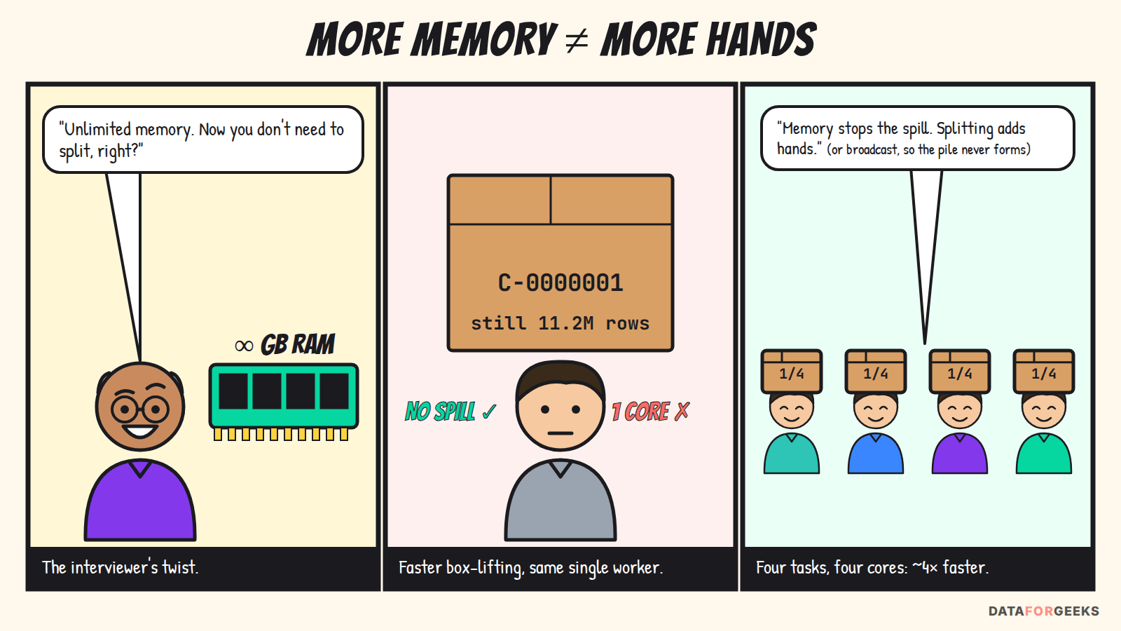
“Forget the budget. Say I give you a cluster with unlimited memory. Would you still split the skewed partition, or just let it run?”

It’s a trap in both directions. “No, memory solves it” shows you think skew is a memory problem. “Yes, always split” without a reason sounds memorised. Here’s how Nikhil answers, one layer at a time.

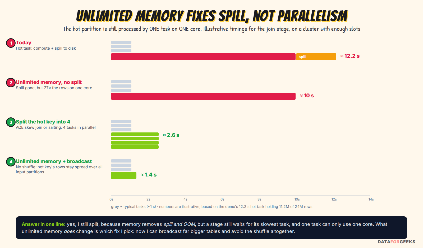
The timings in this image are illustrative, derived from the demo’s measured 12.2 s hot task. The real AQE run earlier reached 7.1 s rather than the ideal ≈ 12 ÷ 4, because each split still spilled and all tasks shared a 2-core laptop. With memory to spare and free cores, splits get close to the ideal.

Short answer: yes, I would still split

“Yes, I’d still split, because memory isn’t the bottleneck; parallelism is. Unlimited memory removes the spill and the risk of an out-of-memory error, but the hot partition is still processed by one task, and one task runs on one core. The stage still waits for that task. Memory makes the slow task a bit less slow; splitting makes it several fast tasks.”

Why memory alone doesn’t fix skew

Go back to the formula: stage time ≈ max(slowest task, total work ÷ slots). Memory doesn’t appear in it. It only changes how long the slowest task takes, and only by the part of that time that was caused by memory:

What the hot task spends time on	Does unlimited memory remove it?
Spilling to disk and merging the spilled runs	Yes: everything fits in memory
Out-of-memory failures and task retries	Yes
Fetching its 92.6 MiB of shuffle blocks	No: same bytes over the network
Sorting / hashing 11.2M rows for the join	No: CPU work on one core
Joining and pre-aggregating 11.2M rows	No: CPU work on one core

In the demo, the hot task handled about 27× the rows of a typical task (11.2M vs about 420k). Take the spill away and it is still doing 27× the work on one core while 31 other cores sit idle. The skew is the same; it just stops spilling.

Two more details an expert would add. First, with memory to spare you can let Spark use a shuffled hash join instead of a sort-merge join (preferSortMergeJoin=false, or AQE’s maxShuffledHashJoinLocalMapThreshold, off by default), which skips the sort. That makes the hot task cheaper, but it’s still one task. Second, “unlimited memory” is never quite free in a JVM: huge heaps full of objects mean longer garbage-collection pauses. Spark’s Tungsten binary format keeps most join and sort data off the object heap, which helps, but it doesn’t make the hot task parallel.

What unlimited memory does change: which fix I choose

This is the part that separates a good answer from a great one. Memory doesn’t remove the need to spread the work, but it changes the cheapest way to do it:

• Broadcast becomes the first choice, even for big tables. With memory to spare on the driver and every executor, I can broadcast a much larger “small” side. Then there’s no shuffle of the big table at all, so the hot key’s rows stay spread across all the input partitions. It isn’t a split; the skew never forms. The limits still apply: Spark’s 8 GB hard limit on a broadcast table, the time to collect it on the driver, and the network cost of sending it to every executor (size × number of executors).
• Fewer, larger partitions become OK for the non-skewed part. Without spill risk, I can raise advisoryPartitionSizeInBytes and let AQE coalesce into fewer, bigger tasks: less scheduling overhead and fewer shuffle files. The limit is parallelism: keep at least as many tasks as task slots, or cores sit idle.
• Caching becomes cheap. If the same input feeds several steps, persist() in memory avoids re-reading it.
• The skewed task itself still gets split (AQE skew join or selective salting) whenever the join has to shuffle.

When I would not split

“Always split” isn’t the right answer either. Splitting has a cost: the other side’s matching partition is copied once per split, and salting adds code to maintain. I’d leave it alone when:

• The cluster has few slots and the total work ÷ slots term already dominates, as on our 4-slot laptop, where skewed and even runs took the same time. Splitting won’t shorten the stage.
• The skewed stage isn’t on the critical path, for example a small side branch that finishes while a bigger stage is still running.
• The hot partition is only modestly bigger (say 2× the median, below AQE’s thresholds). The gain doesn’t pay for the extra copies and tasks.
• A broadcast removes the shuffle entirely. Then there’s nothing to split.

Bonus question: how can AI help you fix this?

The last question of the practice round is a very current one:

“Everyone uses AI assistants now. How would an LLM help you resolve this issue?”

Both easy answers are weak. “I’d paste the error into ChatGPT” sounds like you’d skip the thinking. “I wouldn’t trust AI” sounds out of date. The interviewer wants to know whether you can use AI to go faster without giving up the evidence. Nikhil’s short answer:

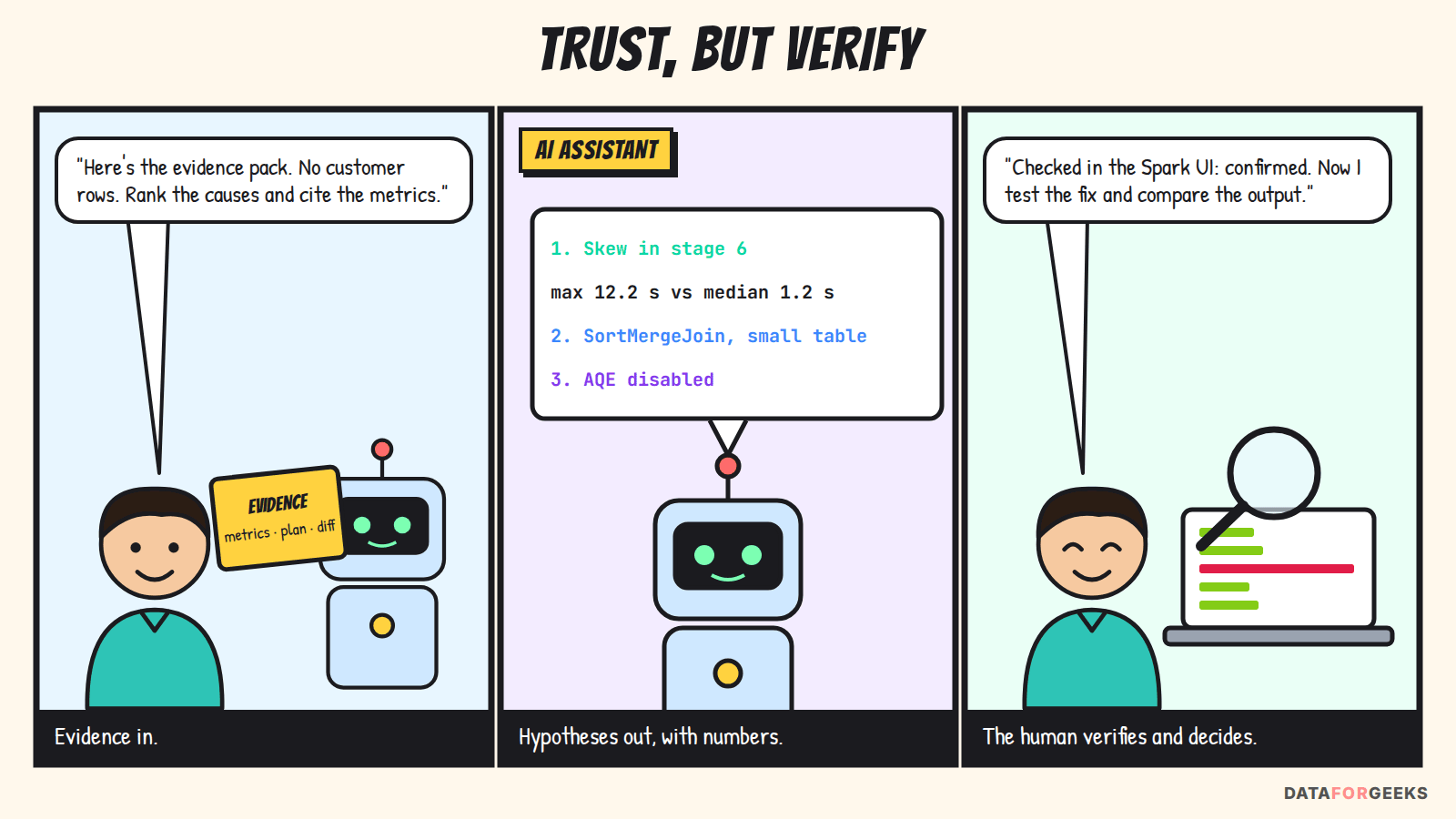
“I’d use it as a fast assistant inside the same debugging loop, not as the one who decides. I give it evidence: stage metrics, the physical plan, the config diff. It gives me ranked hypotheses, explanations and draft code. Then I verify every claim in the Spark UI and test every change, the same as I would with a colleague’s suggestion.”

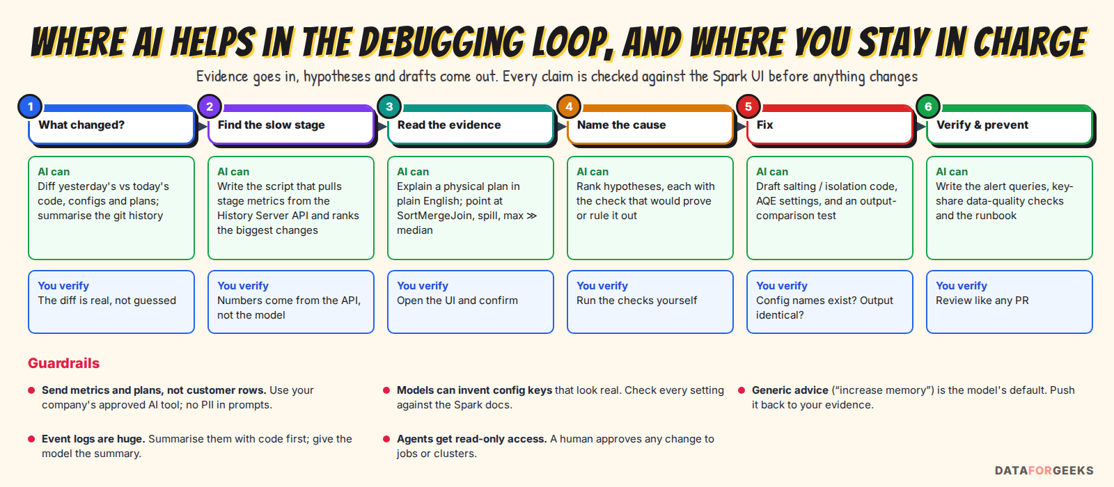
Where AI speeds up each step

• What changed: summarising the git history of the job, and diffing yesterday’s and today’s configs and physical plans. A changed join strategy is easy to miss in two 300-line plans and easy for a model to point out.
• Finding the slow stage: the model doesn’t need to “read” the UI. It writes the script that pulls the numbers from the Spark History Server REST API, and the numbers come from Spark, not from the model.
• Reading the evidence: explaining a physical plan node by node, which is great for less experienced engineers on call at 2 a.m.
• Naming the cause: producing a ranked list of hypotheses, each with the metric that supports it and the check that would rule it out.
• Fixing: drafting the selective-salting or hot-key isolation code, plus a test that compares old and new output on the same input.
• Preventing: writing the runtime alerts, the key-share data quality check and the runbook entry.

The trick is to give the model an evidence pack, not a vague question. A few lines of Python build it from the Spark History Server REST API:

import json, requests

API = "http://<history-server>:18080/api/v1/applications/<app-id>"   # YARN cluster mode: append /<attempt-id>
pack = []
for s in requests.get(f"{API}/stages", params={"status": "complete"}).json():
    q = requests.get(f"{API}/stages/{s['stageId']}/{s['attemptId']}/taskSummary",
                     params={"quantiles": "0.5,1.0"}).json()          # median, max
    pack.append({"stage": s["stageId"], "name": s["name"][:60], "tasks": s["numTasks"],
                 "run_ms_median_max": q["executorRunTime"],
                 "shuffle_read_bytes_median_max": q["shuffleReadMetrics"]["readBytes"],
                 "spill_bytes_median_max": q["memoryBytesSpilled"]})
print(json.dumps(pack, indent=1))    # add: df.explain("formatted") + the config diff

Then ask a question that forces an evidence-based answer:

“A daily Spark job went from 10 to 45 minutes; data grew about 3×. Below are per-stage task metrics for yesterday and today, today’s physical plan, and the config diff. Rank the three most likely causes. For each, quote the exact metric that supports it and the check that would confirm or rule it out. Don’t suggest adding hardware. Only use configuration keys that exist in the official Spark documentation.”

With our demo’s numbers, the pack makes the answer hard to miss: one stage with a 12.2 s max vs a 1.2 s median, a 92.6 MiB partition against a 5.8 MiB median, spill in a single task, and a SortMergeJoin against a small table. A good assistant should reach the conclusion we reached by hand, only faster. That’s the value: speed, not a different answer. And if it reaches a different answer, the metrics it quotes tell you immediately whether to take it seriously.

Tools you can mention

• AWS Apache Spark Troubleshooting Agent (Amazon EMR on EC2, EMR Serverless, EMR on EKS and AWS Glue): works through an MCP-compatible AI assistant in your IDE. It analyses Spark History Server logs, configurations and error traces, and returns root-cause analysis and code or configuration recommendations. It gives recommendations only; you apply and validate them.
• Databricks Assistant: helps explain and fix code and errors inside Databricks notebooks. Pair it with the Spark UI and query profile for the performance evidence.
• Any approved general-purpose assistant: given the evidence pack above, it can do most of the reasoning steps, as long as your company allows the data to be shared with it.

Where AI falls short, and how to stay safe

Risk	What it looks like	Guardrail
No runtime context	Generic advice: “increase executor memory”, “add partitions”	Always attach metrics and the plan; ask it to cite them
Made-up details	Config keys or API fields that look plausible but don’t exist	Check every key in the Spark docs; test in a lower environment
Data exposure	Sample rows with customer IDs or PII pasted into a prompt	Share metrics, plans and schemas, not rows; use the company-approved tool
Too much input	Multi-GB event logs don’t fit in a prompt	Summarise with code first (as above), then send the summary
Unreviewed changes	An agent editing job configs or cluster settings on its own	Read-only access for agents; changes go through code review
Wrong but confident	A plausible diagnosis that the metrics don’t support	Verify in the Spark UI before and after, like any colleague’s suggestion

Summary: Spark performance interview cheat sheet

The two-minute answer

“Since the cost is fixed, I won’t reach for more hardware. I’ll find what changed and where the time goes; 4.5× slower on 3× the data is non-linear, so I suspect skew, spill or a changed join plan. First, what changed: volume, key distribution, code, configs, cluster. Then the Spark UI: the SQL tab to find the query that slowed down, the job’s DAG to find the slowest stage, and that stage’s task quantiles. If max ≈ median, it’s volume, partition count or resources. If max is many times the median in duration and shuffle read, with spill only in the max task, it’s data skew, and the task list and a top-keys query tell me which key.

To fix it without spending more: restore AQE and let it split skewed partitions; broadcast the small table so the big side isn’t shuffled at all; and if both sides are big, isolate or salt the hot keys. If the hot key is junk, filter it and fix upstream. Then I verify the same metrics and add alerts on runtime, input size and top-key share so we hear about it before the business does.”

Cheat sheet

Concept	One-liner
Opening line	Constraint + method + hypothesis, in three sentences
Job / stage / task	Action → job; shuffle → new stage; partition → task on one slot
Stage time	≈ max(slowest task, total task time ÷ slots)
Why one task matters	A stage ends when its slowest task ends
Skew signature	Max ≫ median in duration and shuffle read; spill only at max
Volume signature	All quantiles grow together
AQE	Re-plans after each shuffle: coalesce, switch to broadcast (or shuffled hash join, if enabled), split skew
Skew join rule	Partition > factor (5) × median AND > 256 MB → split to ~64 MB
Broadcast	No shuffle of the big side; default 10 MB threshold, 8 GB hard limit
Salting	Salt hot keys only (hash of a unique column), explode the small side, join on key + salt
Partial aggregation	sum/count already pre-combine; salt only non-combinable aggregates
Spill	Execution memory overflow to disk: a symptom, not a failure. Memory/disk columns are the same data
Unlimited memory?	Removes spill/OOM, not the single slow task; still split, or broadcast so the skew never forms
AI assistants	Evidence in, ranked hypotheses and drafts out; you verify and approve
NULL keys	Inner joins drop them automatically; outer joins need them spread

Common answer vs strong answer

Common answer	Strong answer
Opens with “I’d increase memory.”	Opens with the constraint, a method and a hypothesis to check.
“I’d add executors / memory.”	“One task holds 16× the data; more cores won’t help it. Let me split or avoid that shuffle.”
“I’d check the logs.”	“SQL tab → job → slowest stage → task quantiles → plan → environment.”
“The data grew.”	“Data grew 3×, time grew 4.5×: something non-linear. Quantiles say skew.”
“Use salting.”	“Check for junk keys, then broadcast, then AQE; salt selectively only for big-big joins.”
“Increase shuffle partitions.”	“That helps volume, not skew: the hot key still hashes to one partition.”
“I’d ask ChatGPT.” / “I don’t use AI.”	“I give the model metrics, plan and config diff, it ranks hypotheses, I verify in the UI.”
Stops at the fix.	“Verified with the same metrics, and added alerts on runtime, input size and top-key share.”

Spark performance interview bingo

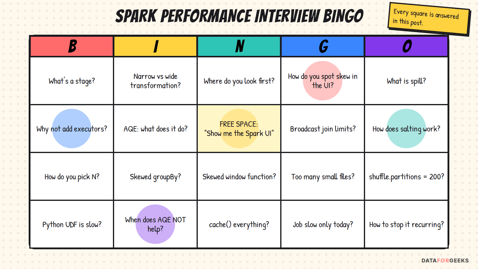
Every square on that card is answered somewhere above. If you can talk through each one with a screenshot in your head, this question stops being scary and becomes one of the best chances in the loop to show how you actually work.

Frequently asked questions

Why is my Spark job suddenly slow?

Usually because something changed: more data, a different key distribution (data skew), a code or config change, a small table that grew past the broadcast threshold, or fewer resources. Compare yesterday’s and today’s runs in the Spark UI, find the stage that got slower, and compare its median and max task metrics.

What is data skew in Spark?

Data skew is an uneven spread of data across partitions, usually because a few join or group-by keys are far more frequent than others. After a shuffle, all rows with the same key land in one partition, so one task does most of the work while the other cores wait.

How do I find data skew in the Spark UI?

Open the slow stage in the Stages tab and read the Summary Metrics. If the max task duration and max shuffle read are several times the median, and spill appears only in the max column, you have skew. The task list shows which partition it is; a groupBy(key).count() shows which key.

How do you fix data skew in Spark?

Cheapest first: make sure AQE and its skew join are on, broadcast the smaller side of the join, filter or spread junk keys such as NULLs, isolate known hot keys on a separate path, and use selective salting for joins where both sides are big.

Does AQE fix data skew automatically?

Partly. AQE’s skew join splits oversized partitions in sort-merge joins when a partition is larger than 5 times the median and 256 MB (defaults). It doesn’t fix skewed aggregations, window functions or writes, skew below the thresholds, or joins where it’s turned off.

What is salting in Spark?

Salting adds a salt value (0 to N-1) to rows with a hot key on the big side of a join, and copies the matching rows N times on the other side, so the hot key is spread over N partitions. Salt only the hot keys and derive the salt from a unique column rather than rand().

Will adding more executors or memory fix a skewed Spark job?

Not by itself. More memory removes spill, and more executors speed up the other tasks, but a skewed partition is still processed by one task on one core. Stage time is roughly max(slowest task, total work ÷ task slots).

What do Spill (memory) and Spill (disk) mean in the Spark UI?

Both describe the same spilled data: Spill (memory) is its size in memory before spilling, and Spill (disk) is its serialized, compressed size on disk. Spill in only one task usually points to data skew.

Further reading on DataForGeeks:

• Apache Spark performance tuning and best practices: the tuning knobs in detail.
• The Vendor Who Pushes: the design half of this practice session.
• One Ride, 400 Milliseconds: a system design and data model walkthrough.