It’s 9:14 PM on a rainy Friday in Bengaluru. Nikita has just wrapped up a long week at work and wants to get home. She taps Request Ride.
Within about 400 milliseconds her request has to be authenticated, rate-limited, priced, safely recorded and handed to dispatch. Within a few seconds, a dozen systems in her region have to agree on who picks her up, what she pays, how long she waits, and what gets written down so it can be audited, analyzed and fed into a model later.
Meanwhile, in a glass-walled meeting room, Nikhil, a senior data engineer, is taking his turn in the candidate’s chair at a system-design practice session with friends. One of them plays interviewer and asks the question that has ended many good interviews. Nikhil is ready for it.
“Design the data model for a ride-hailing app.”
This post follows Nikita’s ride from tap to payment, and then follows the data after she gets home. At each stop we look at the part of the system that handles it, and at the questions an interviewer is likely to ask there: what they’re really testing, what a strong answer sounds like, and the follow-up question that trips people up.
The story is in three acts:
- Act I · The whiteboard: how to run the 45 minutes, requirements, napkin math, the front door (API gateway, rate limiting, load shedding) and the core entities.
- Act II · The ride: real-time matching, race conditions, CAP trade-offs, sharding and scaling, event logs, regions, caching, error handling, IDs and payments.
- Act III · After the ride: the data pipeline, observability and real-time dashboards, the scheduler, the analytics star schema, slowly changing dimensions (SCD Types 1, 2 and 4), and a lightning round of the less common interview questions.
Grab a coffee, maybe two. The ride takes 27 minutes and the interview takes 45. This guide is long because it’s meant to be complete: bookmark it and come back to each act.
Table of Contents
Act I · The whiteboard
Scene 1: The question (a.k.a. the first 5 minutes)
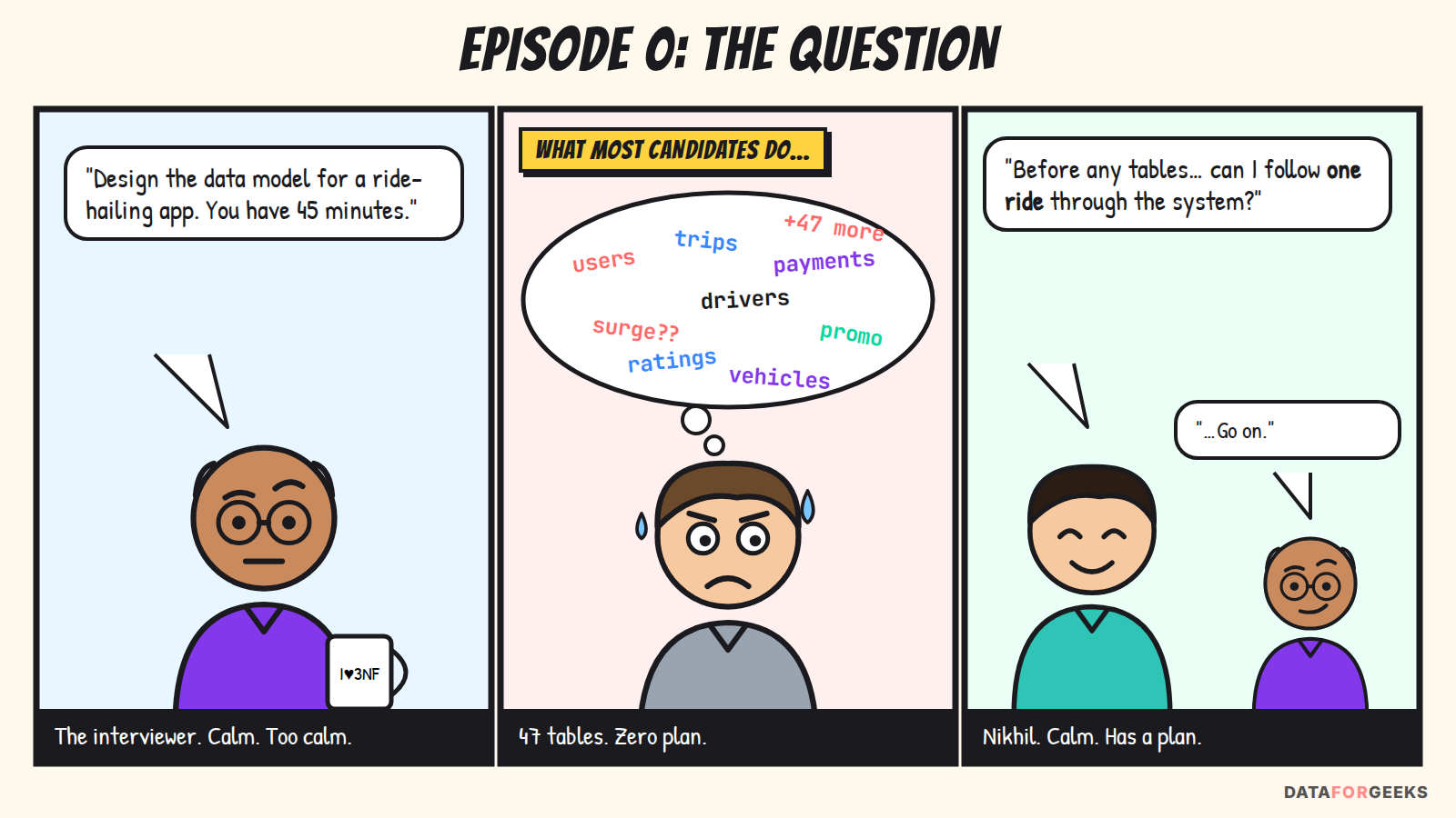
Most candidates stumble in the first five minutes. It isn’t a knowledge problem. They start drawing users, drivers and trips tables before they know what they’re designing for.
Nikhil takes a breath. In a system design round, the strongest candidates drive the conversation instead of waiting for questions. So before anything else, he tells the interviewer how he’ll use the time:
| Minutes | What Nikhil does | What it signals |
|---|---|---|
| 0–5 | Clarify functional and non-functional requirements, scope, assumptions | Handles ambiguity, doesn’t build the wrong thing |
| 5–8 | Napkin math: QPS, storage, hot state | Designs from numbers, not vibes |
| 8–15 | Front door, APIs, service map, high-level data flow | Sees the whole system before zooming in |
| 15–30 | Data model deep dive: entities, keys, events, regions, cache, IDs, payments | Depth where it matters most |
| 30–40 | Scale and failure: sharding, CAP, error handling, observability, scheduling | Thinks about day 2 and 3 AM incidents |
| 40–45 | Analytics model, evolution, trade-offs, what he’d do next | Owns the long-term roadmap |
He also says: “Stop me whenever you want me to go deeper on something. Matching and payments are usually the interesting bits.” Interviewers love that line, because it hands them control while showing that Nikhil knows where the hard parts are.
Then he writes down the requirements in two columns:
| Functional (what it does) | Non-functional (how well) |
|---|---|
| Rider: fare estimate, request, cancel, track, pay, rate, trip history and receipts, schedule a ride | Latency: API p99 < 200 ms; driver matched in a few seconds |
| Driver: go online/offline, stream location, accept/decline, navigate, complete, see earnings and payouts | Availability: 99.99% for booking and trip updates |
| Platform: matching, surge pricing, promos, notifications, fraud checks | Durability: never lose a trip, payment or rating |
| Ops and analytics: real-time city dashboards, reporting, ML (ETA, surge, fraud) | Consistency: strong where money or assignment is involved, eventual elsewhere |
| Compliance: data export, deletion, audit trail | Scale, multi-region, observability, cost-efficiency, security |
Now he sets out the objective: a robust, real-time and analytics-ready data model for a ride-hailing platform that serves millions of users and daily transactions across regions. Then he says his assumptions out loud:
- Actors and roles: riders and drivers are different roles, but both are users.
- Core workflows: the rider requests a ride → the system matches a driver → the trip is tracked in real time → completion and payment → post-trip feedback and ratings.
- Scale and performance: millions of trips a day, high concurrency, users spread around the world.
- Latency: under a second for booking, matching and tracking. Reporting can be batch or near-real-time.
- Compliance and regulation: GDPR, CCPA and India’s DPDP Act. We must support data deletion, anonymization and audit trails.
Next come the architectural principles that every later decision has to follow:
- Real-time readiness: live trip status, driver availability and matching.
- Data lineage: every trip state transition can be traced for audits and debugging.
- Versionability: schema evolution, because vehicle types and pricing strategies will change.
- Event-centric thinking: every major transition is an event, so it can be time-traveled, replayed and analyzed.
- Separation of concerns: transactional data is decoupled from analytical and compliance workflows.
Finally he sketches a first stack, with a one-line reason for each layer:
| Layer | Technology | Purpose |
|---|---|---|
| Operational DB | DynamoDB / PostgreSQL | Scalable, reliable, low-latency reads and writes for mutable state |
| Caching | Redis | Hot data such as active drivers, availability and session cache |
| Streaming | Kafka | Decoupled, async propagation of trip status and events |
| Orchestration | Airflow / Dagster | Workflow scheduling and ETL jobs |
| Storage | S3 + Iceberg / Delta Lake | Scalable analytics, schema evolution, time travel |
| Search | ElasticSearch | Geo-indexing, geospatial lookups, full-text search |
| ML serving | SageMaker / Vertex AI | Fraud detection, ETA prediction, dynamic pricing |
THE INTERVIEWER ASKS
“Before you design anything, what are you assuming?”
What they’re really testing: Can you scope an ambiguous problem, or do you jump straight to tables?
Strong answer: Cover actors, workflows, scale, latency targets and compliance in under two minutes, then say which workflows you’ll go deep on. “I’ll focus on the trip lifecycle and treat payments as a downstream consumer” is a senior-sounding sentence.
Follow-up trap: “Why do you care about compliance in a data model?” Because deletion, residency and audit requirements change your partition keys, what goes in event payloads, and how you keep history (see SCDs in Act III). Adding them later means a rewrite.
THE INTERVIEWER ASKS
“SQL or NoSQL?”
What they’re really testing: Whether you have a favorite tool or can reason from workloads.
Strong answer: “Both, each where it fits.” NoSQL (DynamoDB) gives predictable single-digit-millisecond latency at any scale for known access patterns. SQL (PostgreSQL) gives transactional accuracy, joins and ad-hoc queries, and is often the better home for a payments ledger. A data lake (S3 + Iceberg/Delta) gives cheap, effectively unlimited scale for history and analytics. Say which workload goes where and why.
Follow-up trap: “If you could only pick one OLTP store?” A partitioned PostgreSQL (or a distributed SQL database like Spanner) can handle the whole OLTP layer. What you give up is some operational simplicity at extreme write volumes, especially for location pings.
💡 Interview tip: Align your stack with the problem. Every technology on the whiteboard should come with a reason: NoSQL for low latency, SQL for transactional accuracy, data lakes for scale and cost. Listing tools without reasons is a red flag.
Scene 2: The napkin math
Before choosing between DynamoDB and Postgres or deciding what goes in Redis, Nikhil does what many candidates skip: a quick estimate of scale. These numbers are assumptions stated out loud. The interviewer cares that you can reason with numbers, not that you guess a particular company’s figures.
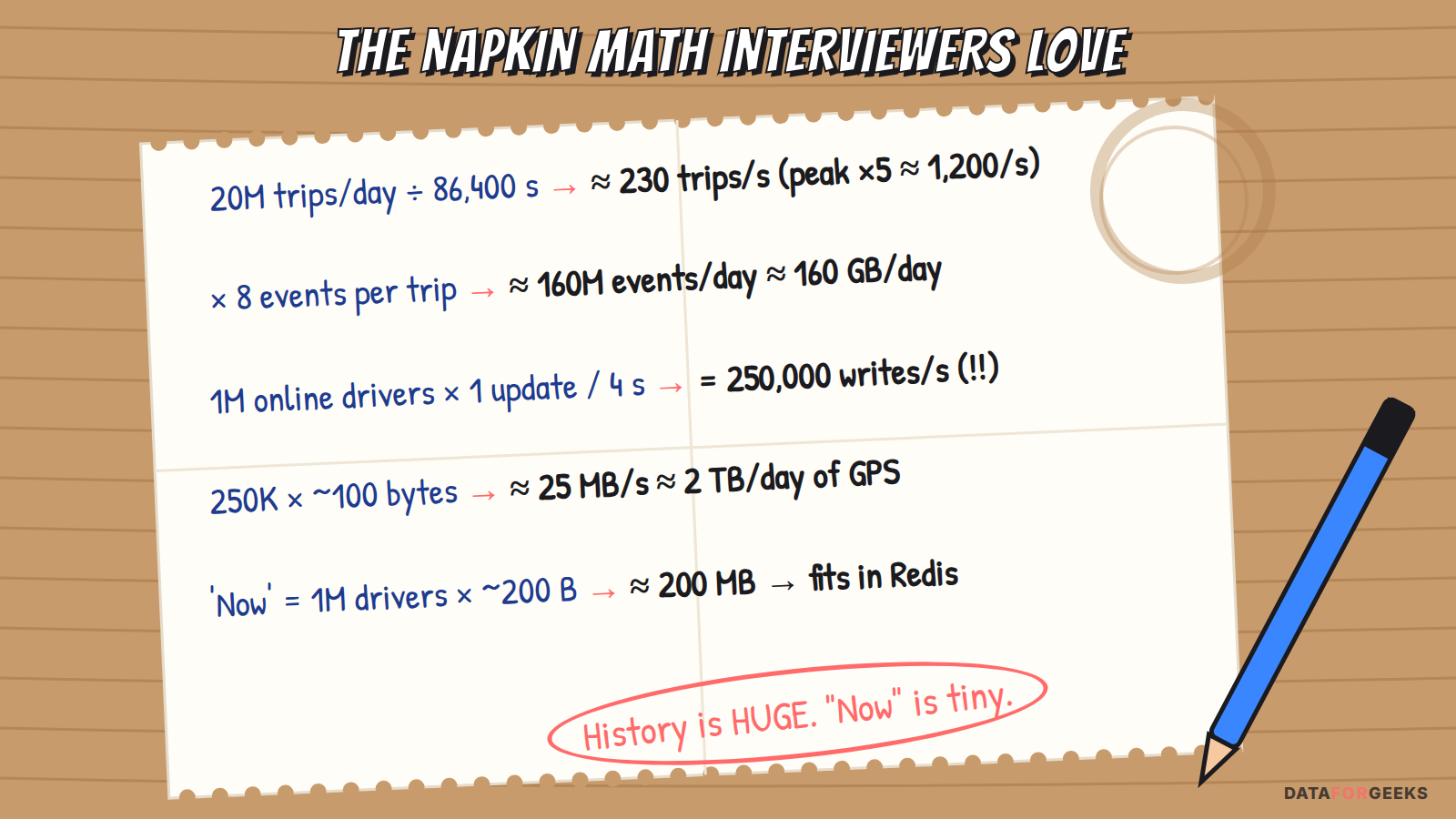
- Trips: 20M/day ÷ 86,400 s ≈ 230 trips/s on average, and about 1,200/s at a 5× peak. That’s modest.
- Trip events: about 8 per trip → 160M/day. At ~1 KB each that’s ~160 GB/day.
- Location pings: 1M online drivers × 1 location update every 4 s (each a small batch of GPS fixes) = 250,000 writes/s. This is the real firehose.
- GPS volume: 250K × ~100 bytes ≈ 25 MB/s ≈ 2 TB/day, or roughly 800 TB/year before compression.
- Live state: 1M online drivers × ~200 bytes (position, status, current trip) ≈ 200 MB. It fits comfortably in Redis memory.
The napkin gives Nikhil his main design insight: history is huge, and “now” is tiny. The current state of the world (who’s online, where, doing what) is small and very hot, so it belongs in memory. The history is enormous and cold, so it belongs in cheap, partitioned storage with TTLs in the OLTP layer. The rest of the design follows from those two facts.
THE INTERVIEWER ASKS
“Roughly how much data are we talking about?”
What they’re really testing: Can you size a system, and do the numbers change your design?
Strong answer: Walk through the napkin, then draw conclusions. Trip writes are easy. Location writes need an append-only, partitioned, TTL’d store and a stream. Live state fits in memory. GPS history must be compacted and tiered in the lake.
Follow-up trap: “And at 10× growth?” Trip writes are still fine. Location writes reach 2.5M/s, so you’d shard location ingestion by region and H3 cell, sample or aggregate pings on the device (for example, send less often when the car is stationary), and keep raw GPS in the OLTP layer for only a short time.
Scene 3: The front door (API gateway, rate limiting, load shedding)
“Walk me through what happens when Nikita taps the button,” says the interviewer. Nikhil starts at the edge, because every request passes through the front door before any data model sees it, and the front door is what keeps the data layer alive on a bad night.
The path of one tap
- DNS / global load balancing: latency-based or geo DNS (or anycast) sends Nikita to the nearest healthy region,
ap-south. - Edge / CDN: terminates TLS close to her, and applies WAF rules, DDoS protection and bot detection. Static assets and map tiles are served from cache.
- Regional L7 load balancer: spreads traffic across availability zones and gateway instances, and runs health checks.
- API gateway: the bouncer and receptionist (details below).
- Services: synchronous gRPC/REST on the request path, Kafka events for everything that can happen asynchronously.
- A real-time channel: a persistent WebSocket / gRPC stream through a connection gateway carries driver location pings up and trip updates down (“Ravi is 2 min away”). Mobile push (APNs/FCM) is the fallback when the app is in the background.
What the API gateway does, and what it deliberately doesn’t
| Does ✅ | Doesn’t ❌ |
|---|---|
| Authentication (OAuth2 / JWT validation), coarse authorization | Business logic (fares, matching, trip rules) |
| Rate limiting and quotas per user, device, IP and endpoint | Talk to databases |
| Request validation, payload size limits, schema checks | Hold state (it must be stateless so it scales horizontally) |
Routing, API versioning (/v1), canary and traffic splitting | Become a “god service” every team edits |
Requires an Idempotency-Key header on POSTs, injects request ID and trace context | |
| Protocol translation (REST ↔ gRPC), timeouts, circuit breaking to upstreams |
The service map
Behind the gateway, each service owns its data (database-per-service). No other service reaches into its tables; they call its API or consume its events:
- Rider BFF / Driver BFF: backend-for-frontend layers shaped for each app.
- Location service: ingests pings and maintains the Redis geo index and the location stream.
- Dispatch / matching: finds and ranks candidates and makes the conditional assignment.
- Trip service: owns the trip state machine and
trips/trip_events. - Pricing: fare estimates, surge and promos.
- Payments: the ledger, the payment gateway integration and payouts.
- Notification, Identity, Ratings, Fraud: supporting services.
The APIs (a quick sketch)
| Endpoint | Purpose | Notes |
|---|---|---|
POST /v1/fare-estimates | Price quote | Returns quote_id, locks surge for ~2 min |
POST /v1/rides | Request a ride | Idempotency-Key required; body includes quote_id |
GET /v1/rides/{ride_id} | Ride status | Served from Redis read-through |
WS /v1/rides/{ride_id}/stream | Live updates | Driver position, ETA, state changes |
POST /v1/rides/{ride_id}/cancel | Cancel | State-machine guarded, may add a fee |
POST /v1/drivers/me/locations | Location pings | Batched (one call every ~4 s with the latest few GPS fixes), high rate limit |
POST /v1/rides/{ride_id}/rating | Rate | One per side per trip |
POST /v1/scheduled-rides | Book ahead | See Chapter 13 |
Rate limiting: the token bucket at the door
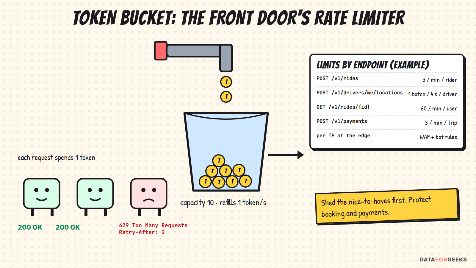
At 9:10 PM a concert ended at the stadium three kilometres from Nikita’s office. Forty thousand people opened the app at the same moment, some of them tapping “Request” over and over. Without a rate limiter, that turns into a self-inflicted DDoS.
| Algorithm | How it works | Good | Watch out |
|---|---|---|---|
| Fixed window | Count per minute, reset on the minute | Dead simple | Bursts at window edges (2× traffic across a boundary) |
| Sliding log | Keep a timestamp per request | Exact | Memory-hungry at scale |
| Sliding window counter | Weighted blend of current and previous windows | Accurate enough, cheap | Approximate |
| Token bucket | Tokens refill at rate r, up to capacity b; each request spends one | Allows short bursts, smooth average; industry default | Tune b and r per endpoint |
| Leaky bucket | Queue drains at a constant rate | Smooths output to downstream | Adds queueing delay |
Where to limit: in layers. Per IP and bot rules at the edge, per user/device/API key and per endpoint at the gateway, and per-dependency concurrency limits inside services.
How to make it distributed: keep counters in Redis and update them atomically with a small Lua script (read tokens, refill based on elapsed time, decrement, set TTL, all in one round trip). At very high QPS, gateways keep local buckets and sync to Redis periodically, trading a little precision for far fewer network hops. Responses use 429 Too Many Requests with Retry-After and X-RateLimit-* headers so well-behaved clients back off.
Load shedding and backpressure: protect what matters
Rate limiting protects you from one noisy client. Load shedding protects you from everyone arriving at once. Nikhil assigns priorities:
- P0, never shed: ride requests, trip state changes, payments, safety features.
- P1, degrade gracefully: live tracking frequency (every 4 s becomes every 8 s), ETA refinements.
- P2, shed first: trip history, promo carousels, recommendations, analytics beacons.
Techniques: adaptive concurrency limits per service, queues with deadlines (drop work whose client has already timed out; serving a dead request is pure waste), autoscaling on RPS and queue depth, and pre-scaling for known peaks such as New Year’s Eve, festivals and large concerts.
THE INTERVIEWER ASKS
“Design a distributed rate limiter for this API.”
What they’re really testing: Algorithms, distributed-state trade-offs, and failure behavior.
Strong answer: Token bucket keyed by (user_id | device_id | ip, endpoint), state in Redis updated by an atomic Lua script with a TTL, limits loaded from config so they can change without a deploy, 429 + Retry-After. Layered: edge (IP/bot), gateway (user/endpoint), service (concurrency). Local token caches for hot paths.
Follow-up trap: “The rate limiter’s Redis is down. Fail open or fail closed?” It depends on the endpoint. Fail open (with conservative local limits) for ride requests, because blocking all bookings is worse than a few extra requests. Fail closed for login, OTP and payments, where abuse is expensive. Saying “it depends, and here’s the rule” is the strongest answer.
THE INTERVIEWER ASKS
“It’s New Year’s Eve. At 00:00 traffic jumps 20×. Walk me through it.”
Strong answer: Before: pre-scale stateless tiers, pre-warm caches, raise DynamoDB capacity or confirm on-demand headroom, freeze deploys, prepare runbooks. During: rate limits and priority-based shedding protect P0, surge pricing balances demand and supply (that’s what it’s for), tracking frequency degrades, and dashboards (Chapter 12) watch match rate and p99 per city. After: scale down gradually and review which limits triggered. The data model helps too: region and cell sharding keep a Mumbai spike from affecting Delhi.
THE INTERVIEWER ASKS
“A buggy app release makes 50,000 drivers send location pings every 100 ms.”
Strong answer: Per-driver rate limits on the location endpoint absorb it (1 batch / 4 s; excess gets 429 or is sampled). The location service drops or downsamples surplus fixes instead of queueing them. Kafka quotas protect the brokers. Dashboards show pings per driver per app version, so the bad release is identified in minutes, and a feature flag or remote config tells the clients to slow down, so you aren’t waiting on an app-store review. Blast radius: zero for riders.
Scene 4: Meet the cast
Only now does Nikhil draw entities. Because he knows the workflows and the scale, he can explain each one in terms of how it is used.
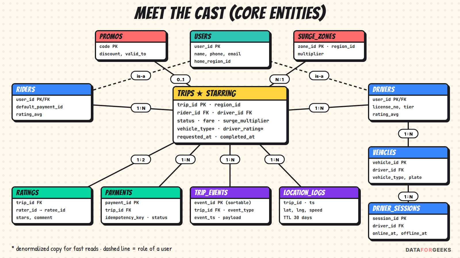
usersholds shared identity and PII.ridersanddriversare role tables keyed on the sameuser_id. The same person can be both, which is why “is-a” beats two unrelated tables.tripsis the central entity: one row per trip with its current state. It is deliberately denormalized, copyingvehicle_typeanddriver_ratingas they were at booking time.trip_eventsis the append-only history of every state change (Chapter 5).trip_location_logsholds the GPS trail of trips in progress. It’s the highest-volume table and has a TTL. Off-trip pings (drivers cruising) only go to Redis and Kafka → lake; writing all 250K/s into DynamoDB would be needlessly expensive.vehiclesanddriver_sessionsrecord what a driver drives and when they were online.paymentsandratingsrecord money and feedback, and both carry compliance and refund obligations.promosandsurge_zonesare pricing inputs, with hot copies in Redis.
With DynamoDB you design keys from access patterns, not from entities. Nikhil writes the access patterns next to the tables:
| Access pattern | Table / index | Partition key | Sort key |
|---|---|---|---|
| Get a trip by ID | trips | region_id#trip_id | (none) |
| Rider’s trip history, newest first | trips GSI-1 | rider_id | requested_at#trip_id |
| Driver’s trip history | trips GSI-2 | driver_id | requested_at#trip_id |
| All events of a trip, in order | trip_events | region_id#trip_id | event_id (time-sortable) |
| GPS trail of a trip | trip_location_logs | region_id#trip_id | ts (+ TTL) |
| Driver’s online sessions | driver_sessions | region_id#driver_id | online_at |
| Payment for a trip (dedupe) | payments | trip_id | payment_id |
THE INTERVIEWER ASKS
“Walk me through your entities. Why is a driver not just a column on users?”
What they’re really testing: Basic modeling judgment: roles versus identities, and normalization versus denormalization.
Strong answer: Identity and PII belong in one place (users), which also makes GDPR erasure a single, contained job. Role-specific attributes (license, tier, payment method) live in role tables, so one person can be both a rider and a driver. The trip record then deliberately denormalizes a few attributes for fast reads.
Follow-up trap: “You copied vehicle_type into trips. Isn’t that redundant?” It’s a snapshot, not a mistake: it records what was true when the trip happened. If the driver changes car tomorrow, last week’s trips should still say hatchback. That’s the same idea behind SCD Type 2 in Act III.
Act II · The ride
Chapter 1 · 9:14:02 PM: Nikita taps “Request”
The first thing the system needs is available drivers near Nikita, right now. It sounds simple, and it’s where a lot of designs fall over.
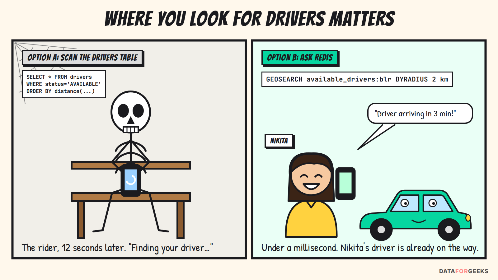
If you answer “we query the drivers table”, your rider ends up like the skeleton on the left. Luckily, Nikita is riding on Nikhil’s design. The napkin already told us why the table scan is wrong: 250,000 location updates a second, read thousands of times a second per city. That’s an in-memory workload.
Nikhil applies the first two operational design principles:
- Low latency first: optimize for fast matching, live driver updates and rider notifications. Use DynamoDB or Redis for latency-critical lookups, and keep read/write paths for real-time entities under 100 ms where feasible.
- Cache what you query frequently: real-time availability, trip status and driver state hit Redis first. Use TTLs and pub/sub for invalidation and synchronization, and don’t cache cold, low-value entities, so memory is kept for hot data.
How it works: each driver’s app sends a location update every few seconds. The location service writes it to a geo index, available_drivers:<region> (a Redis geo set, which is a sorted set underneath). At scale that key is split per H3 cell, available_drivers:<region>:<cell>, because one Redis key lives on one shard (Chapter 4). One subtlety interviewers like: Redis TTLs expire whole keys, not individual members of a set. So the service also keeps a companion sorted set scored by last-ping time, and a sweeper removes drivers who haven’t pinged for ~30 s (ZRANGEBYSCORE + ZREM), while driver_state:<driver_id> hashes carry their own TTL. Nobody gets matched with a driver whose phone died. Candidates are ranked by proximity and recency: a driver 400 m away who pinged 2 s ago beats one 300 m away whose last ping was 25 s ago. In practice, “proximity” means road-network ETA from a routing engine, not straight-line distance. A driver 300 m away across a river or on the wrong side of a flyover can be ten minutes out.
THE INTERVIEWER ASKS
“Why not just query the database for the nearest drivers?”
What they’re really testing: Do you design around access patterns or around entities?
Strong answer: Driver location is high-churn and short-lived and it’s read constantly, which makes it a textbook in-memory workload. Redis gives sub-millisecond geo queries (GEOSEARCH), and a last-ping sweeper removes stale drivers. The database stores sessions (driver_sessions) and trails (trip_location_logs) for audit. It doesn’t store the live dot on the map.
Follow-up trap: “Where does ElasticSearch fit, then?” For richer geospatial and full-text lookups (search by landmark or address, filter by vehicle type or accessibility), not the tight matching loop.
Chapter 2 · 9:14:05 PM: Two riders, one driver
Ravi, a driver two streets away, is the best match for Nikita. He’s also the best match for Karan, who tapped “Request” at the same millisecond from the café next door.
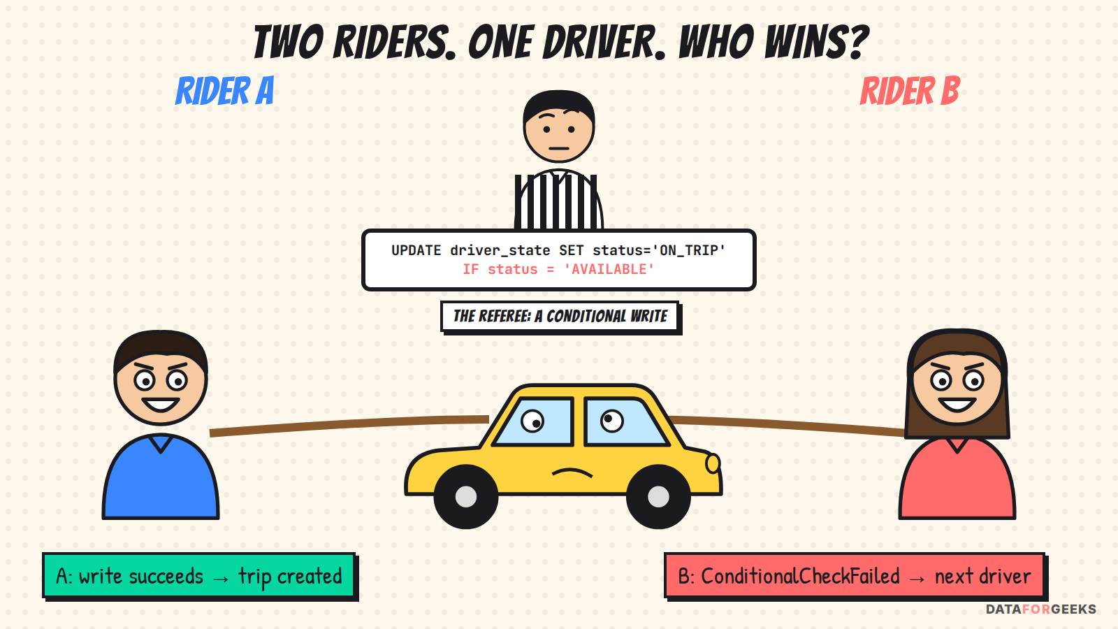
This is the question that separates people who have built these systems from people who have only drawn them. Only one booking can win, and the database should enforce that, not luck.
Nikhil’s answer is a conditional write on the source of truth: set Ravi to ON_TRIP only if he’s still AVAILABLE. In DynamoDB that’s a ConditionExpression (or a TransactWriteItems call that creates the trip and flips the driver’s state atomically). In Postgres it’s UPDATE … WHERE status = 'AVAILABLE' with a row count check. The losing request gets a clean failure and moves on to the next driver. Tonight Nikita’s write lands first, and Karan gets matched with a driver 90 seconds away. Nobody is double-booked and nobody is left stranded.
One more real-world detail: the driver has to accept. Dispatch doesn’t just assign Ravi; it offers the trip to him. The conditional write puts him in OFFERED (a short reservation, e.g. 15 s, so no one else can offer him a trip), his app shows the request, and only his tap moves the trip to ACCEPTED. If he declines or the offer times out, the reservation is released and the next candidate gets the offer. Large platforms also batch matching: instead of greedily giving each rider the nearest driver, they collect requests for a second or two and solve a small assignment problem, which lowers the total pickup time across all riders.
This follows the operational flow using Redis from the design:
- The rider starts a booking, and the service checks
available_drivers:<region>. - Candidate drivers are ranked by proximity and recency.
- The booking is confirmed with the conditional write in DynamoDB (durable path, source of truth), then
trip_status:<trip_id>anddriver_state:<driver_id>are updated in Redis (hot path). - The change is persisted to downstream systems through the dual-write / change-stream pattern, and notifications go out: “Ravi is on the way”.
- TTLs clean up expired and inactive keys.
THE INTERVIEWER ASKS
“You write to Redis and DynamoDB. What if one succeeds and the other fails?”
What they’re really testing: Do you understand that dual writes aren’t atomic?
Strong answer: Write DynamoDB first with the conditional check, because it’s the truth. Update Redis second. If the cache update fails, the trip still exists. Redis TTLs plus a change stream (DynamoDB Streams → Kafka) repair the cache, and readers fall back to DynamoDB on a miss. Make every write idempotent (keyed on trip_id) so retries are safe. For the strongest guarantee, use the transactional outbox pattern (write the change and an outbox record together, then publish from the outbox) or rely on CDC so that “write to DB” and “publish event” can never diverge.
Follow-up trap: “Why not write to Redis first, since it’s faster?” Because then a crash leaves a trip that exists only in a cache that is designed to forget it (see Chapter 7).
Chapter 3 · 9:14:06 PM: The consistency dial (CAP, for real this time)
The interviewer leans back: “You keep saying ‘source of truth’ and ‘strong consistency’. Is your system CP or AP?”
This is the CAP theorem question, and there’s a trap in it. Quick recap: when a network partition (P) happens, a distributed system has to choose between consistency (C), where every read sees the latest write or gets an error, and availability (A), where every request gets an answer even if it’s stale. You can’t avoid partitions, so the real choice is C or A when things break.
The trap is answering for the whole system. Nikhil’s answer is “it depends on the operation“, and he backs it up:
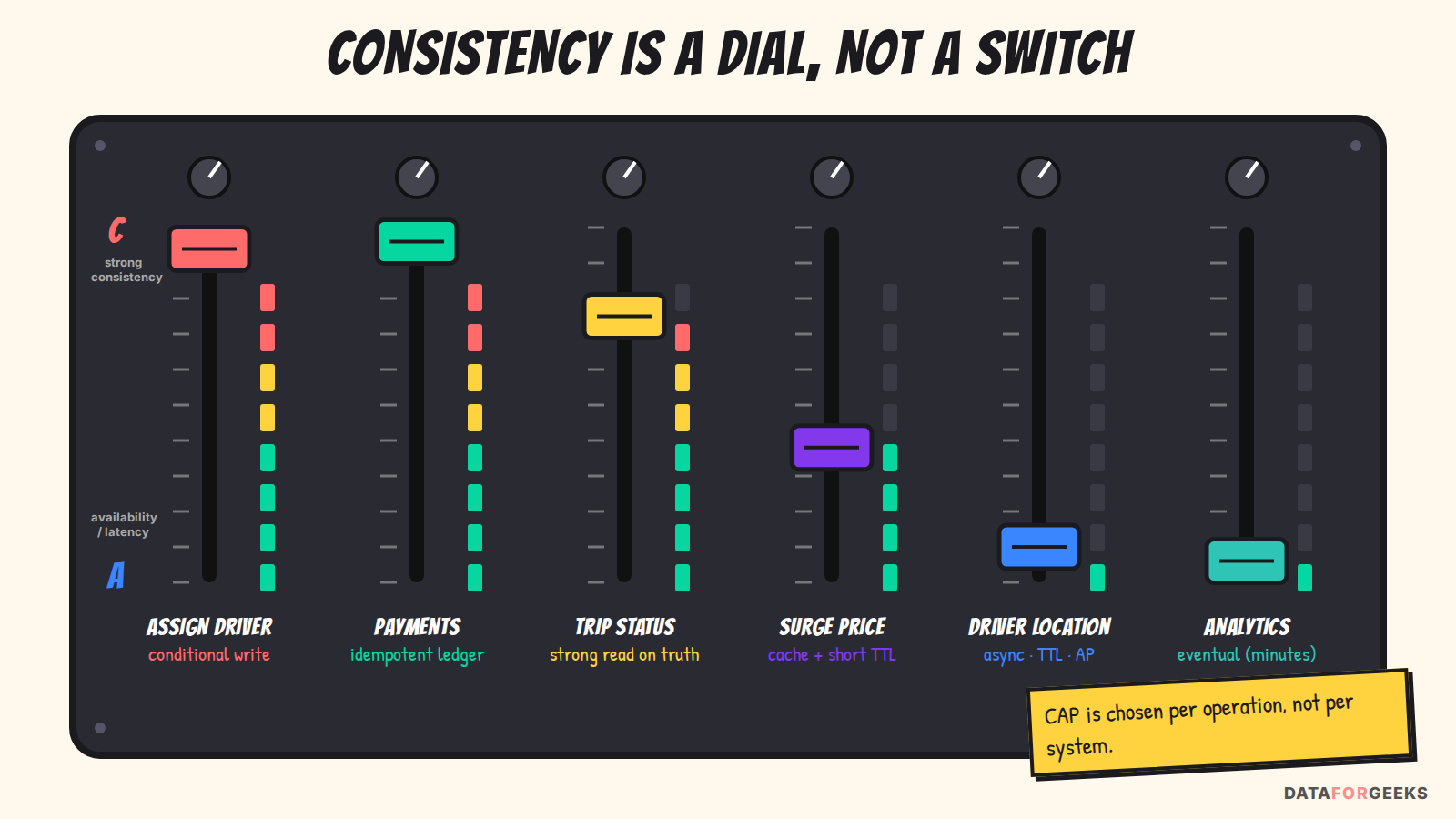
| Operation | Choose | Why | How |
|---|---|---|---|
| Assign driver to trip | C | A double-booking is worse than a 200 ms retry | Conditional write / transaction on DynamoDB, strongly consistent read |
| Payments | C | Money. Enough said. | Idempotency keys, ACID ledger, reconciliation |
| Trip status (for the apps) | C-leaning | The rider and driver must agree on the state | State machine with conditional transitions; Redis is a read-through copy |
| Surge multiplier | A, bounded staleness | A few seconds stale is acceptable; the value shown is locked into the quote | Redis with short TTL; the multiplier used is logged in the trip event |
| Driver location on the map | A | A dot that’s 3 s stale is fine. A blank map isn’t. | Redis, async replicas, TTLs |
| Ratings, history, analytics | A / eventual | Seconds or minutes of lag is fine | Eventually consistent reads, GSIs, streams → lake |
A strong answer also mentions PACELC: if there’s a Partition, choose A or C; Else, choose Latency or Consistency. Even when nothing is broken, strong consistency costs latency. DynamoDB reflects this directly: reads are eventually consistent by default (cheaper and faster), strongly consistent reads are opt-in per request on the base table, and GSIs only support eventually consistent reads. That’s why the “assign driver” check reads the base table, never a GSI.
Across regions, DynamoDB Global Tables replicate asynchronously by default (multi-Region eventual consistency, with last-writer-wins on conflicts). Since mid-2025 there’s also a multi-Region strong consistency (MRSC) mode that offers a zero recovery point objective (RPO) at the cost of higher write latency. Nikhil’s design avoids needing it for most data by homing each trip in one region (Chapter 6), so two regions never compete to write the same trip.
THE INTERVIEWER ASKS
“So, is your system CP or AP?”
What they’re really testing: Whether you understand CAP as a per-operation trade-off or just recite it.
Strong answer: “Neither as a whole. It’s a dial per operation.” Then give the table above in 30 seconds: CP for assignment and payments, AP for location, surge and analytics, with the mechanism for each. Mention PACELC to show you know the everyday trade-off is latency versus consistency, not just partitions.
Follow-up trap: “The Booking API loses its connection to DynamoDB in the middle of an assignment. What does Nikita see?” The assignment is CP, so the system refuses rather than guesses. Nikita sees “Finding your driver…” for another moment while the request retries with the same idempotency key. The map (AP) keeps showing nearby cars from Redis. Degrading the “nice to have” features while protecting the critical ones is what the interviewer wants to hear.
THE INTERVIEWER ASKS
“Two regions write to the same row at the same time. What happens?”
Strong answer: With default Global Tables, the last writer wins and one update is silently lost, which is unacceptable for trips or money. So avoid multi-region writers by design: every trip, payment and driver session is homed in one region, and other regions read replicas. Where a single entity truly needs global strong consistency (for example, a global wallet balance), use MRSC or a single-writer service and accept the latency.
Chapter 4 · 9:14:10 PM: The stadium hexagon (sharding and scaling)
Nikita is lucky: her office is three kilometres from the stadium. The 40,000 concert-goers are not so lucky. They’re all asking for rides from one small patch of the map. The interviewer smiles: “A big chunk of Bengaluru’s traffic just landed in one spot. Now what?”
This is where sharding goes from a buzzword to a design decision. First, the vocabulary. Partitioning splits data into pieces. Sharding is partitioning across machines. Vertical splitting separates by table or service. Horizontal splitting separates rows of the same table. Region partitioning (Chapter 6) is the outermost horizontal split. Inside each region you need a second level.
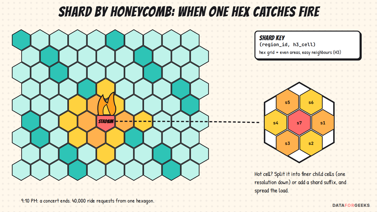
Sharding strategies, and where each fits
| Strategy | How | Good for | Risk |
|---|---|---|---|
| Hash | hash(key) mod N or consistent hashing | Even spread: trips, payments, users | Range scans become scatter-gather |
| Range | Key ranges per shard (e.g. by time) | Time-series scans, archives | “Latest” range becomes a hot shard |
| Geo | Cell of a spatial index (H3 / geohash / S2) | Driver supply, location, surge, matching | Dense cells (stadiums, airports) get hot |
| Directory / lookup | A lookup table maps key → shard | Moving tenants or cities between shards | Directory becomes a dependency; cache it |
| Composite | (region_id, hash or cell) | Most tables here | More moving parts |
For geo, Nikhil picks H3, the open-source hexagonal hierarchical spatial index that Uber built. Hexagons have uniform neighbors (every neighbor is the same distance away, unlike squares’ diagonals), and the index is hierarchical, so a hot cell can be broken into finer child cells at the next resolution. That’s exactly what the stadium needs.
Shard key per table
| Data | Shard key | Why |
|---|---|---|
| Driver supply / geo index (Redis) | (region, h3_cell@res7) | Matching queries a cell plus its neighbors (k-ring) |
trips, trip_events | (region, hash(trip_id)) | Even writes; all events of a trip are colocated |
trip_location_logs | (region, trip_id) + time sort key | Append-only, read per trip |
payments / ledger | (region, account_id) | Balance queries stay on one shard |
| Kafka topics | Message key = trip_id (or driver_id) | Per-key ordering, parallel consumers |
| Redis Cluster | 16,384 hash slots; hash tags like {trip_id} | Keeps related keys in one slot for multi-key operations |
Taming the hot shard
- Split the cell: move the stadium cell to a finer H3 resolution so its load spreads across 7 child cells and more shards.
- Salt the key: append a suffix
0..Nto spread writes, and scatter-gather on read (fine for a few hot keys). - Cache and coalesce: 40,000 people asking “what’s the surge here?” should become one computation served from cache, not 40,000.
- Pre-warm for known events: concerts have calendars. Raise capacity and pre-position driver incentives before the encore.
- Let the platform help: DynamoDB’s adaptive capacity and automatic partition splitting absorb a lot of skew, but you still shouldn’t design a key that routes a whole city to one partition.
Scaling the whole system, not just the database
- Stateless services behind load balancers, autoscaled on RPS, CPU and queue lag.
- Cell-based architecture: each region is split into independent cells (a full stack serving a slice of users or cities). A bad deploy or a poison request hurts one cell, not the region. Roll out cell by cell.
- CQRS and read replicas: writes go to the source of truth; read-heavy views (trip history, receipts) come from replicas, GSIs or materialized views.
- Async by default: anything not needed to answer the user right now (receipts, analytics, loyalty points) goes through Kafka.
- Capacity planning: start from the napkin, validate with load tests (including replaying last NYE’s traffic shape), and keep headroom targets per tier.
THE INTERVIEWER ASKS
“How would you choose the shard key for driver locations?”
What they’re really testing: Do you derive the key from the query?
Strong answer: The dominant query is “drivers near point P”, so shard by geo cell (H3) within a region. The matching service queries the rider’s cell plus its k-ring of neighbors. Driver ID lookups use a separate driver_state:<driver_id> key. That’s two access patterns with two keys, which is normal.
Follow-up trap: “A driver drives across a cell boundary every minute. Isn’t that a lot of moves?” Yes. It’s a cheap delete-and-insert in memory, done on each ping. It’s why the geo index lives in memory and not in a durable table.
THE INTERVIEWER ASKS
“You need to go from 16 to 64 shards. No downtime. How?”
Strong answer: Ideally you planned for this with many logical shards mapped onto fewer physical nodes (e.g. 4,096 logical shards on 16 machines), so resharding means moving logical shards rather than rehashing every key. Otherwise: (1) dual-write to old and new layouts, (2) backfill historical data, (3) verify with row counts and checksums, (4) shadow-read and compare, (5) cut over reads behind a flag, (6) stop the old writes and clean up. Consistent hashing with virtual nodes limits how much data moves.
THE INTERVIEWER ASKS
“Show me all trips for a rider across shards.”
Strong answer: Don’t scatter-gather in OLTP for a user-facing screen. Maintain a secondary index keyed by rider_id (the GSI from Scene 4) or a per-rider materialized view fed by events. For cross-rider or cross-region questions, go to the lake or OLAP store. Scatter-gather is acceptable only for rare admin tools.
THE INTERVIEWER ASKS
“What’s a cell-based architecture and why would you use it here?”
Strong answer: A cell is a complete, independent copy of the stack serving a fixed slice of traffic, with a thin routing layer that pins each user or city to a cell. Benefits: limited blast radius (a poison message or bad deploy hits ~5% of users, not 100%), predictable scaling (add cells), and safer rollouts. It’s partitioning applied to the whole system, not just the data.
Chapter 5 · 9:19–9:41 PM: The ride and its paper trail
Ravi arrives at 9:19. Nikita gets in at 9:20. They reach home at 9:41. Across the company, other teams will ask a lot of questions about this ride. Why was the pickup slow? Did the surge price apply correctly? Why do cancellations spike in Koramangala at 6 PM?
If all you stored was trips.status = 'COMPLETED', you can’t answer any of them.
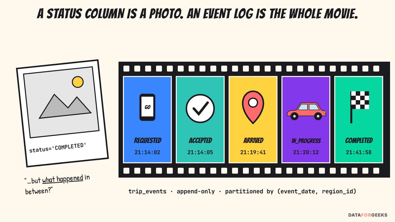
This is the heart of the design: an immutable, append-only trip_events log. Every transition (requested → accepted → arrived → in progress → completed, or cancelled at any point) becomes a new row. You never update a row and you never lose one. It gives you time-travel, debugging, process mining and SLA audits, and it’s partitioned by event_date and region_id so analytics can scale.
CREATE TABLE trip_events (
    event_id    VARCHAR(26) NOT NULL,  -- time-sortable (ULID / Snowflake)
    trip_id     VARCHAR(26) NOT NULL,
    region_id   VARCHAR(16) NOT NULL,  -- partition key, always present
    event_type  VARCHAR(32) NOT NULL,  -- REQUESTED | ACCEPTED | CANCELLED | ...
    seq_no      INT         NOT NULL,  -- per-trip sequence, detects gaps/reordering
    actor_type  VARCHAR(16),           -- rider | driver | system
    actor_id    VARCHAR(26),
    payload     JSON,                  -- fare, location, reason codes, surge used
    event_ts    TIMESTAMP   NOT NULL,  -- UTC, event time (not arrival time)
    event_date  DATE        NOT NULL,  -- lake partition column
    PRIMARY KEY (region_id, trip_id, event_id)
);
The trip itself is a state machine, and the Trip service enforces its legal transitions with conditional writes. COMPLETED → ACCEPTED is rejected, and a late duplicate ARRIVED is ignored thanks to seq_no.
Three more operational principles apply here:
- Write-aware modeling:
trip_events,trip_location_logsanddriver_sessionstake heavy write traffic. Make them append-only (less locking, faster inserts), use compound keys like(region_id, entity_id)to avoid hotspots, and add TTL indexing where the data is short-lived. - Minimize joins on real-time APIs: denormalize critical entities, storing vehicle type and driver rating inline in the trip record, so the “Your ride” screen doesn’t need a five-way join.
- Versionability: keep rapidly evolving attributes in a JSON
payload, so a new vehicle type or pricing strategy doesn’t require a migration.
💡 Interview tip: Don’t leave design principles abstract. Tie each one to a specific entity or feature (“append-only because trip_location_logs takes 250K writes/s”). That shows your design is practical and extensible.
THE INTERVIEWER ASKS
“Why an event log? Isn’t a status column simpler?”
What they’re really testing: Event-centric thinking. Do you design for the questions people will ask later, not just today’s screen?
Strong answer: A status column records the latest state and overwrites everything before it. An event log keeps the full history, so you get time-travel, replay, debugging, process mining and SLA audits. Keep both: trips holds current state for fast reads, and trip_events holds the history. The current state can even be rebuilt from the log.
Follow-up trap: “Is this event sourcing, then?” Partly. Full event sourcing makes the log the only source of truth and derives all state from it, which adds complexity (snapshots, replays, versioned event schemas). Here the event log is authoritative for history, and the trips row is a maintained projection for speed. Saying where you stop is itself a senior answer.
THE INTERVIEWER ASKS
“Give me cancellation rate by city for the last 7 days.”
SELECT t.pickup_city,
       COUNT_IF(e.event_type = 'CANCELLED') * 1.0
     / NULLIF(COUNT_IF(e.event_type = 'REQUESTED'), 0) AS cancel_rate
FROM   silver.trip_events e
JOIN   silver.trips t USING (region_id, trip_id)
WHERE  e.event_date >= current_date - INTERVAL 7 DAYS   -- partition pruning
GROUP  BY t.pickup_city;
Point out that event_date partitioning makes this cheap (that’s why you chose it), and ask one clarifying question: “Cancelled by whom? Rider cancels and driver cancels mean very different things.” Asking that kind of clarifying question is what experienced engineers do.
THE INTERVIEWER ASKS
“Events for a trip arrive out of order. What breaks?”
Strong answer: Nothing, if you planned for it. Kafka guarantees order per partition, and idempotent producers keep that order even across retries, so keying by trip_id keeps one producer’s events in order. But a trip’s events come from several services (the driver app, dispatch, payments), and failed events get re-published later, so consumers still check seq_no and the state machine: stale transitions are ignored, gaps are held briefly or fetched from the source of truth. Analytics always uses event_ts (event time), never arrival time.
THE INTERVIEWER ASKS
“Product launches auto-rickshaws tomorrow. What changes in your schema?”
Strong answer: Very little, by design. vehicle_type is a value, not a column per type. Type-specific attributes go in the JSON payload, Kafka schemas evolve in a backward-compatible way via a schema registry, and the lake uses Iceberg/Delta schema evolution to add columns without rewriting data. The fact that this question is boring to answer shows the design works.
Chapter 6 · Meanwhile, in Paris…
At the same moment, Léa is booking a ride in Paris. Her data is protected by GDPR, and it shouldn’t cross the Atlantic just because a US server was less busy. Nikita’s data falls under India’s DPDP Act. A user in California is covered by CCPA.
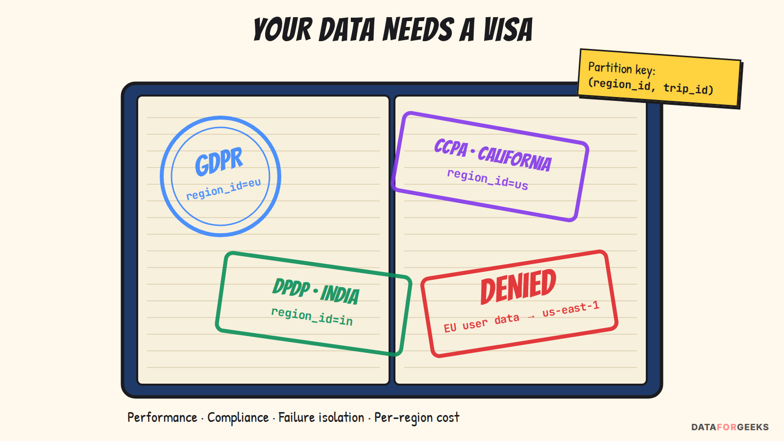
This is why Nikhil partitions by region from day one, even if the company launches in a single city.
- Performance optimization: Nikita’s request shouldn’t make a round trip to Virginia.
- Scalability: each region is an independent unit of horizontal scale, so tables, services and streams shard cleanly.
- Data residency and compliance: GDPR (EU) and DPDP (India) may require data to stay within certain borders.
- Failure isolation: an APAC incident shouldn’t affect US-West.
- Cost optimization: each region can have its own retention, storage and compute policies.
Implementation looks the same at every layer:
region_idis a mandatory column and partition key in high-traffic tables (trips,driver_sessions,trip_events).- OLTP stores such as DynamoDB or Spanner use compound keys:
(region_id, entity_id). - Lake folders are partitioned by a
/region_id=…/prefix for efficient query pruning. - Kafka topic keys include
region_idfor parallel, regional consumption.
There are two options. Option 1 is a single table with a region_id column as a prefix or partition key (e.g. trip_id = apac#TRIP1234 or a (region_id, trip_id) compound key). Option 2 is separate tables per region (trips_us, trips_apac). Recommendation: use a single table partitioned by region_id unless legal or compliance rules require physical separation.
💡 Interview tip: Point out that regional partitioning goes beyond data modeling. You are engineering for resilience, compliance and scalability at a global scale.
THE INTERVIEWER ASKS
“Nikita flies to Paris for a well-earned holiday and books a ride there. Which region owns her data?”
Strong answer: Split it. Her profile stays in her home region under its residency rules. The trip belongs to the region where it happens, because that’s where the driver, pricing, local regulations and latency are. The trip references her by user_id and carries only the minimum PII the local operation needs (e.g. first name for the driver). A small global directory maps user_id → home_region so any region can route profile lookups.
THE INTERVIEWER ASKS
“What happens when an entire region goes down?”
Strong answer: Define RPO (how much data you can lose) and RTO (how fast you recover) per data class first. Trips in flight: the apps retry against a standby region that has replicated state (Global Tables, cross-region Kafka mirroring). Some in-flight trips may need manual reconciliation, and the event log makes that possible. Payments: RPO zero (sync or MRSC-style replication, or a single-writer ledger with synchronous standby). Analytics: hours of RPO are fine. Then say the honest part: failover must be practiced (game days), or it doesn’t work when you need it.
Chapter 7 · 9:22 PM: A Redis node goes down
Nikita is two minutes into her ride when a Redis node in the Bengaluru cluster fails. On-call gets paged. Nikita doesn’t notice anything.
That’s because Nikhil designed around one simple idea:
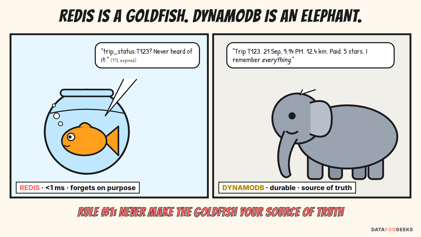
Redis is the goldfish: live, in-memory data for frequent reads and writes, evictable after the session. DynamoDB is the elephant: persistent, durable, queryable, the source of truth.
Why Redis? It’s an in-memory store with under 1 ms latency. It supports rich data structures (hashes, sorted sets, TTLs) and has built-in TTL expiry for automatic eviction. It’s easy to shard with Redis Cluster across zones, scales well with clustering and sharding, and has Pub/Sub for real-time notifications between components.
| Data | Redis key | Structure | TTL? | Purpose |
|---|---|---|---|---|
| Available drivers | available_drivers:<region> | Sorted / geo set | ✅ | Match nearest drivers by location and timestamp |
| Trip status | trip_status:<trip_id> | Hash | ✅ | Current state, ETA, participants |
| Driver state | driver_state:<driver_id> | Hash | ✅ | Login status, current trip, location |
| Surge pricing zones | surge:<region>:<zone_id> | Hash / Set | ✅ | Dynamic pricing multipliers |
| Promo code cache | promo:<code> | String | ✅ | Fast promo validation |
Why DynamoDB? It’s a fully managed NoSQL store with high throughput. It scales horizontally with high write volumes, offers strong consistency when required (payments, trip lifecycle), supports TTL for automatic deletion of stale records, provides Global Tables for multi-region sync, and has DynamoDB Streams to track and stream change events.
| Use case | Table | Why it must be durable |
|---|---|---|
| Trip records | trips | Long-lived trip metadata, cost, IDs |
| Driver sessions | driver_sessions | Audits and session tracking |
| User profiles | users, drivers | Must persist across sessions |
| Payments and feedback | payments, ratings | Compliance and refund tracing |
Integration strategy (hot path + durable path):
- Read path: always check Redis first for live status; on a cache miss, fall back to DynamoDB and optionally repopulate the cache.
- Write path: update DynamoDB (durable) and Redis (hot) to get low latency and auditability.
- Expiry and cleanup: Redis TTLs clear expired data; DynamoDB TTL purges stale records.
- Change streams: DynamoDB Streams or Kafka react to writes and sync downstream systems.
Best practices:
- Sync model: write-through (writes go to both stores) for trip start and trip end; read-through (cache filled lazily when Redis is cold).
- TTL and expiration: set TTLs on ephemeral keys to avoid memory pressure; use an eviction policy (LRU/LFU) plus per-region quotas; use DynamoDB TTL to clean up stale trips and sessions.
- Failover and reliability: Redis is not a source of truth, so if it fails, everything must degrade gracefully to DynamoDB. Redis failover relies on replication, sharding and zonal redundancy, and application logic should detect stale or inconsistent Redis state.
THE INTERVIEWER ASKS
“Redis dies mid-trip. What happens to Nikita?”
What they’re really testing: Do you know which component is the source of truth, and does your system degrade gracefully?
Strong answer: Nothing is lost, because Redis was never the source of truth. A replica is promoted in seconds. Meanwhile reads fall back to DynamoDB, the cache refills lazily, and the geo index rebuilds itself from the next round of driver pings, which arrive within about 4 seconds.
Follow-up trap: “When the cache comes back empty, won’t every request hit DynamoDB at once?” Yes, that’s the thundering herd / cache stampede. Fixes: request coalescing (one loader per key, the rest wait), TTL jitter so keys don’t expire together, a short “stale-while-revalidate” window, and a rate-limited warm-up.
THE INTERVIEWER ASKS
“What’s your cache invalidation strategy?”
Strong answer: TTLs for things that expire naturally (location, surge). Write-through for critical transitions (trip start/end). CDC-driven invalidation (DynamoDB Streams → consumer deletes or refreshes keys) for everything else, plus pub/sub to fan updates out to connection gateways. Don’t cache cold, low-value data.
The line to use in your interview: “I treat Redis as the nervous system of live trip activity: ephemeral but responsive. DynamoDB is the spine: strong, centralized and built for consistency. Together they cleanly separate real-time and durable responsibilities, and the two-layer design also supports elasticity, compliance and global distribution, which are critical for ride-hailing at scale.”
Chapter 8 · 9:26 PM: The promo service hiccups (error handling)
Six minutes into the ride, the promo service starts timing out: a bad deploy on another team. Nikita’s fare needs a promo check at the end of the trip. Does her ride break?
Not in Nikhil’s design, because he treats failure as normal. He sorts failures into categories first: transient (timeouts, throttling, 503s: retry), permanent (validation errors, 4xx: don’t retry, fix the input), partial (one step of a multi-step flow succeeded), poison (a message that fails every time), and duplicate or out-of-order delivery (normal in distributed systems).
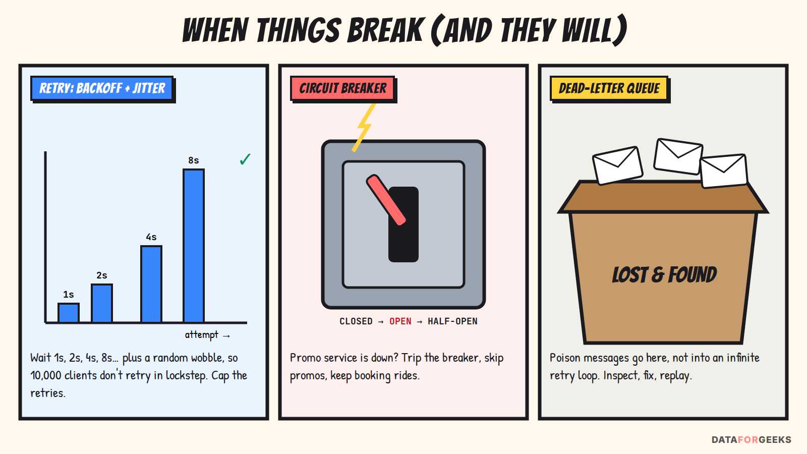
The error-handling toolkit
- Timeouts and deadlines everywhere: every call has a timeout, and the request’s overall deadline is propagated (if 600 ms of an 800 ms budget is used up, downstream calls get only 200 ms).
- Retries, done safely: only for idempotent operations, with exponential backoff plus jitter, a max attempt count, and a retry budget (e.g. retries may add at most 10% extra load). Retry at one layer only: if three layers each make 3 attempts, one failing call can turn into 27.
- Circuit breakers: after N failures the breaker opens, calls fail fast, and after a cool-down it goes half-open to test recovery.
- Bulkheads: separate connection and thread pools per dependency, so a slow promo service can’t use up the resources the payment call needs.
- Fallbacks and graceful degradation: no promo service → finish the trip at the standard fare and apply the promo later as a credit. No fresh surge → use the quoted surge. No ETA model → use a straight-line estimate.
- Messaging safety: at-least-once delivery with idempotent consumers (dedupe on
event_id), a dead-letter queue with alerting and replay tooling, and a transactional outbox for DB-plus-event atomicity. - State-machine guards: illegal or stale transitions are rejected, not “fixed up” silently.
Sagas: long workflows without distributed transactions
Completing a trip touches several services: finalize fare → apply promo → charge rider → credit driver payable → send receipt. A two-phase commit across all of them would be fragile and slow. Instead, use a saga: a sequence of local transactions, each with a compensating action (a refund reverses a charge; a reversing ledger entry cancels a credit). You can run it as orchestration (a workflow engine like Temporal or AWS Step Functions drives each step, which is easier to see and retry) or choreography (each service reacts to the previous event, which is looser but harder to follow). For money, Nikhil prefers orchestration.
THE INTERVIEWER ASKS
“The payment succeeds, but the Trip service crashes before recording it. Now what?”
What they’re really testing: Partial failure and recovery in a distributed workflow.
Strong answer: The saga orchestrator persisted “charge requested with key K” before calling the gateway. On restart it resumes the workflow and retries the charge with the same idempotency key. The gateway returns the original success, and the trip is marked paid. A nightly reconciliation job compares the ledger with gateway settlement files to catch anything that slipped through. No double charge and no lost payment.
THE INTERVIEWER ASKS
“One Kafka message makes your consumer crash every time. What happens?”
Strong answer: Without protection, the consumer crash-loops and that partition stalls, so every trip behind it waits (head-of-line blocking). With protection: bounded retries → move to a DLQ with the error and offset → alert → continue processing. Engineers inspect the message, fix the bug or the data, and replay from the DLQ. Log the poison message’s trip_id so support can see the impact.
THE INTERVIEWER ASKS
“A retry storm took down your database last month. How do you prevent it?”
Strong answer: Jittered backoff, retry budgets, one retry layer, circuit breakers, and load shedding at the gateway. Also server-side signals: return 429/503 with Retry-After so clients slow down instead of hammering the database. Add a dashboard for retry rate per dependency; retries spike before outages do.
Chapter 9 · What’s this ride’s name?
Nikita’s trip needs an ID, and so do the millions of other rides happening at the same moment across dozens of regions.
Suppose you use the familiar auto-incrementing integer:
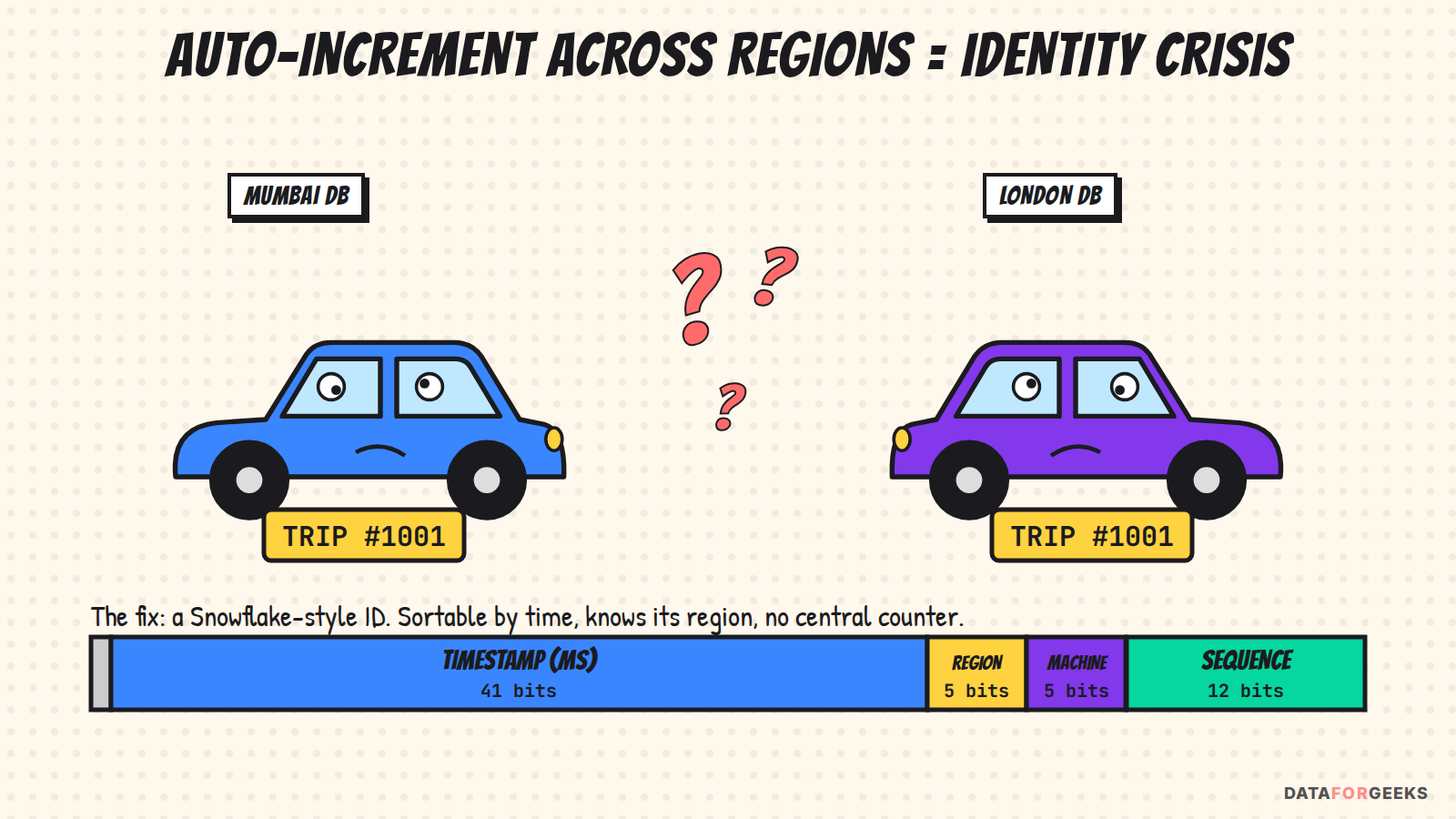
Mumbai issues trip #1001. London issues trip #1001. Now every join, dashboard and Kafka consumer downstream has a problem. At this scale a global ID strategy has to prevent duplicates across services and regions, sort naturally by time, support partition pruning and efficient scans in analytics, and fit event-driven architectures and OLTP systems, all without central coordination.
| Strategy | Good | Bad | Use it for |
|---|---|---|---|
| UUIDv4 (random 128-bit) | No coordination required | Not time-sortable; poor performance in range scans | External identifiers, or where sort order doesn’t matter |
Snowflake-style [timestamp][region_id][machine_id][sequence] | Time-sortable, compact, region-aware; great for OLTP tables and distributed logs | Requires a custom ID service or client-side library | trip_id, payment_id, event_id |
| ULID | Lexically and temporally ordered; decentralized and URL-safe; works with NoSQL and logs | Slightly longer string representation | Event logs, NoSQL sort keys |
Prefixed sequential (apac-0000012345) | Human-friendly | Collision risk and scalability limits without coordination | Low-velocity entities or internal labels only |
Integration considerations: use Snowflake-style IDs or ULIDs for high-throughput, sortable, distributed needs (trip_id, payment_id, event_id). Redis keys and Kafka partitions can embed region and time window for locality. In DynamoDB, use them as range (sort) keys for efficient scans. In Kafka, embed part of the ID in the message key for sharding. Ensure IDs are monotonic within a generator so sort order holds.
THE INTERVIEWER ASKS
“Why not just use UUIDs everywhere?”
Strong answer: UUIDv4 is random. It scatters inserts across the index, can’t be sorted by time, and makes range scans and partition pruning painful. A time-sortable ID sorts in creation order, which helps databases, streams, log correlation and debugging all at once. (UUIDv7 is a time-ordered UUID that gets you most of this in standard UUID format.)
Follow-up trap: “A server’s clock jumps backwards. What happens to your Snowflake IDs?” The generator must detect it and either wait or refuse to issue IDs until the clock catches up, with NTP keeping drift small. The sequence bits handle bursts within a millisecond.
💡 Interview tip: Discuss your ID strategy beyond the database: how it supports stream processing, auditing, log correlation and resilience during network partitions.
Chapter 10 · 9:41 PM: Nikita pays
Nikita gets home, pays ₹248 and gives Ravi five stars. For her it’s one tap. For the platform, it’s the most carefully engineered 300 milliseconds of the night, because a mistake here costs real money.
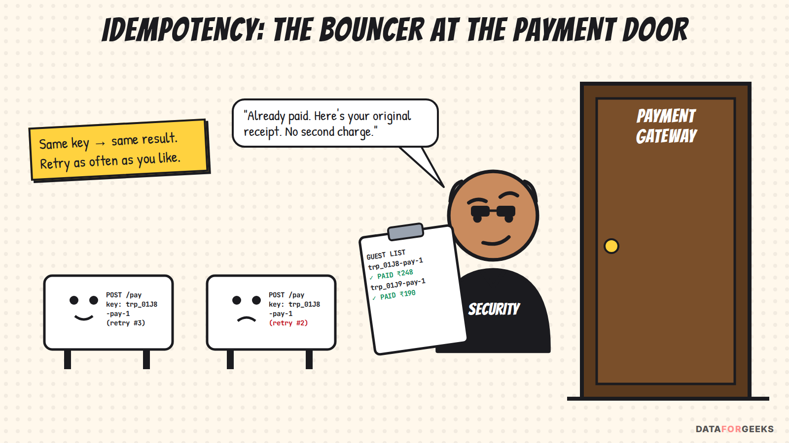
Idempotency keys are the bouncer at the payment door. Every charge attempt carries a key (e.g. trip_id + attempt_no). The payments service first does a conditional insert of that key. If the key already exists, it returns the original result instead of charging again. Network retries, app retries and saga retries all become harmless.
The money itself lives in a double-entry ledger. It’s append-only: every transaction writes balanced entries, so debits always equal credits:
ledger_entries(entry_id, txn_id, account_id, direction, amount, currency, created_at)

txn_42 (Nikita's ride, ₹248):
  DEBIT   rider:nikita.wallet_or_card     248.00
  CREDIT  platform:revenue                 49.60   -- commission
  CREDIT  driver:ravi.payable             198.40
-- refunds and corrections are NEW reversing entries, never UPDATEs
A payment moves through its own state machine: INITIATED → AUTHORIZED → CAPTURED → (REFUNDED | CHARGEBACK), with every transition logged. Many teams keep the ledger in PostgreSQL (ACID transactions, constraints, easy reconciliation queries) even when trips live in DynamoDB. Choosing the right store per workload is a sign of experience.
THE INTERVIEWER ASKS
“The payment gateway times out. Did we charge Nikita or not?”
What they’re really testing: Handling the “unknown outcome” problem, the hardest case in payments.
Strong answer: A timeout means “unknown”, not “failed”. Don’t charge again blindly. Mark the payment PENDING_CONFIRMATION, then (1) retry with the same idempotency key if the gateway supports one (many do; otherwise send a unique merchant order ID per attempt and look it up), or (2) query the gateway’s status API. If it’s still unknown, let reconciliation against the gateway’s settlement report settle it within hours. Nikita never sees a double charge, and Ravi still gets paid.
THE INTERVIEWER ASKS
“Is Kafka ‘exactly-once’ enough for payments?”
Strong answer: Kafka’s idempotent producers and transactions give exactly-once processing within Kafka (read → process → write to Kafka). As soon as you call an external system (a card network, a bank), you’re back to at-least-once, so end-to-end correctness comes from idempotent consumers + idempotency keys + reconciliation. “Effectively once” is the honest term.
THE INTERVIEWER ASKS
“How do refunds work in an append-only ledger?”
Strong answer: Write new reversing entries that reference the original txn_id, and never update or delete. Balances are sums of entries (with periodic snapshots for speed). Auditors can see every step, and “what was the balance on 3 March?” is just a query.
Act III · After the ride
Chapter 11 · 9:42 PM: The ride ends, the data keeps going
For Nikita the story is over, and she’s home. For the data platform, most of the work is just starting. Here’s everything built so far, drawn as a metro map. Follow any colored line and you’re following one piece of Nikita’s ride:
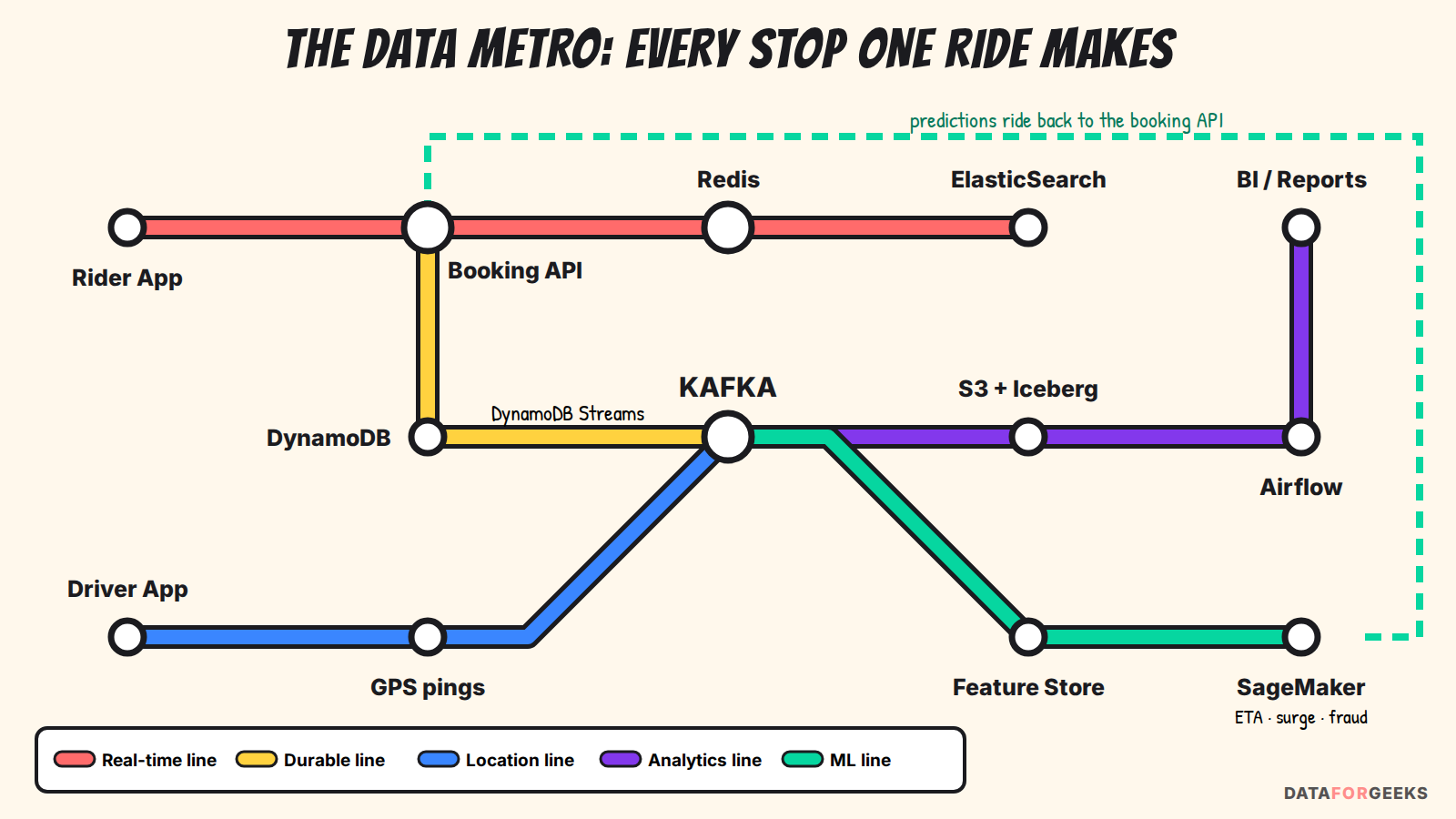
- Real-time line (red): Rider App → Booking API → Redis → ElasticSearch. Matching in milliseconds.
- Durable line (yellow): Booking API → DynamoDB → DynamoDB Streams → Kafka. The source of truth publishes every change (CDC).
- Location line (blue): Driver App → GPS pings → Kafka. The 250K writes/s firehose.
- Analytics line (purple): Kafka → S3 + Iceberg/Delta → Airflow/Dagster → BI. Cheap storage, time travel, schema evolution.
- ML line (green): Kafka → Feature Store → SageMaker/Vertex AI for ETA prediction, surge pricing and fraud detection. Predictions loop back to the Booking API for the next rider.
The lake uses a medallion layout. Bronze holds raw events exactly as received, kept for replay. Silver is cleaned, deduplicated, conformed and SCD-managed. Gold holds business-ready facts and aggregates. Tables are Iceberg/Delta, partitioned by event_date and region_id, compacted hourly (the small-files problem is real at 250K events/s), with GPS tiered to colder storage after 90 days.
This is the separation of concerns principle in action: transactional, analytical and compliance workloads never compete for the same resources, and Kafka connects them all.
THE INTERVIEWER ASKS
“GPS pings from a tunnel arrive 10 minutes late. Does your pipeline break?”
Strong answer: No. Every event carries its own event_ts (event time), and pipelines process by event time, not arrival time. Streaming jobs use watermarks with allowed lateness, and anything later than that goes to a late-data side output. Lake tables are partitioned by event_date, so late data lands in the correct partition through an Iceberg/Delta MERGE or partition overwrite. Airflow backfills are idempotent (re-running a day gives the same result).
THE INTERVIEWER ASKS
“Léa invokes her right to be forgotten. Your event log is ‘immutable’. Now what?”
Strong answer: Keep PII out of event payloads from the start. Events reference user_id, and PII lives in a few profile tables (the Type 1 tables in Chapter 15). Erasure then means deleting or anonymizing those rows, running row-level deletes in Iceberg/Delta for lake copies (followed by snapshot expiry, so old snapshots don’t keep the data), and optionally crypto-shredding (encrypt PII with a per-user key and delete the key). Regional partitioning keeps the job scoped to one jurisdiction. “Immutable” means no business updates; compliance erasure is a documented exception.
THE INTERVIEWER ASKS
“How does surge pricing get computed?”
Strong answer: Flink computes a windowed ratio of demand (REQUESTED events) to supply (available drivers) per H3 cell every few seconds. The ML model adjusts it using features such as weather, events and historical patterns. The multiplier is written to surge:<region>:<zone_id> in Redis with a short TTL, and locked into the fare quote the rider accepts. The multiplier actually used is logged in the trip event, so pricing is auditable and regulators can see exactly why a fare was 1.4×.
THE INTERVIEWER ASKS
“How do you know the lake is correct?”
Strong answer: Data contracts (schemas in a registry, owned by the producing team, with compatibility checks in CI). Automated checks on freshness, volume, nulls, uniqueness and distribution drift. Reconciliation: daily trip counts and revenue in the lake must match the OLTP and ledger totals within a tolerance. Lineage (e.g. OpenLineage) so you know which dashboards break when a table does.
Chapter 12 · Mission control: observability and real-time dashboards
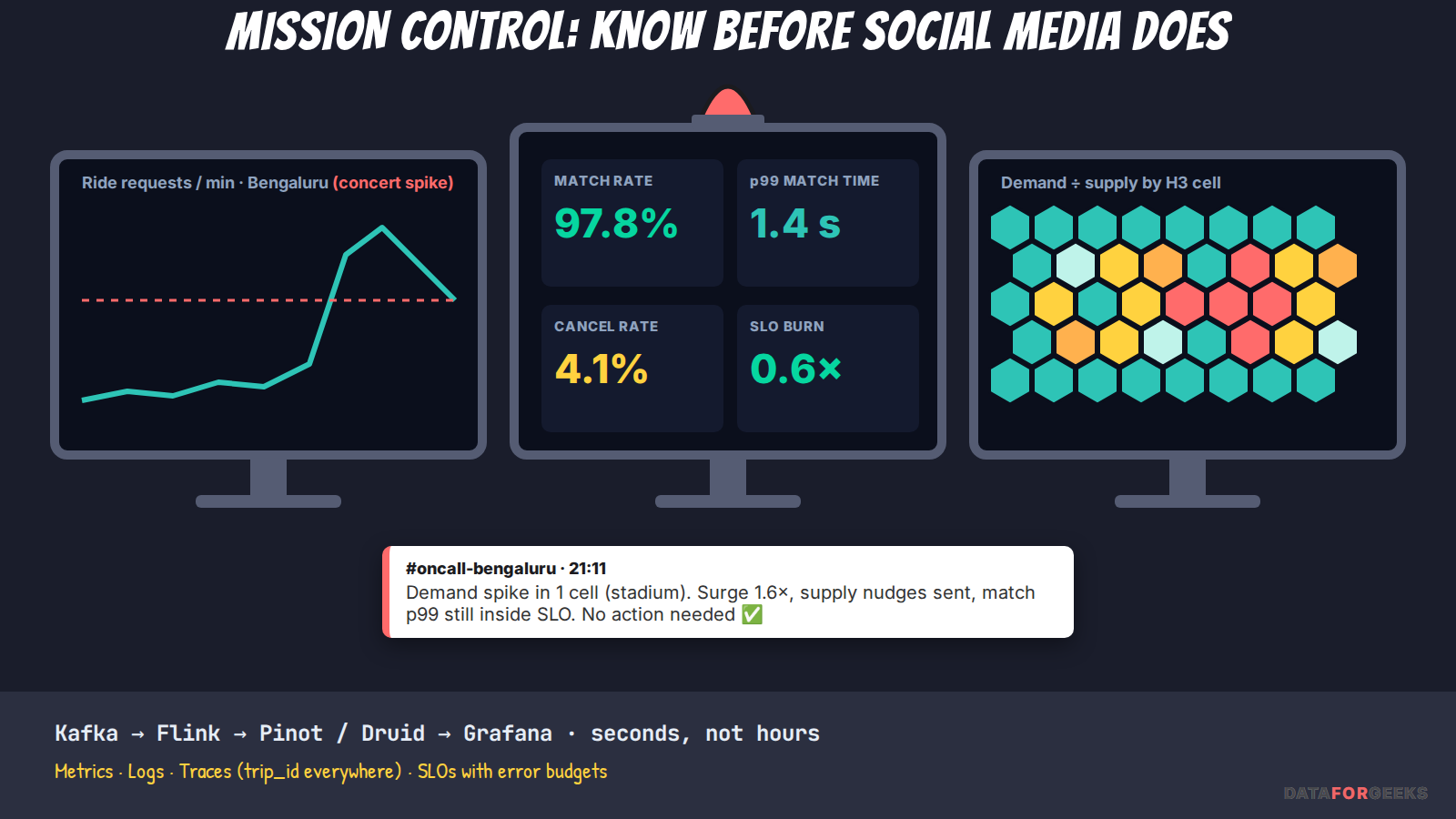
At 9:11 PM, before Nikita even left her desk, an alert fired in #oncall-bengaluru: demand spike in one cell (stadium). Surge went up, supply nudges went out to nearby drivers, and the match p99 stayed inside the SLO. No human had to do anything. That’s what good observability looks like: you know before your users do, and most of the time the system already reacted.
Layer 1: system observability (is the platform healthy?)
- Metrics: the four golden signals (latency, traffic, errors, saturation) per service and endpoint; RED (rate, errors, duration) for services; USE (utilization, saturation, errors) for infrastructure; plus Kafka consumer lag, Redis hit rate and DynamoDB throttles.
- Logs: structured JSON, sampled on success and complete on errors, with PII masked.
- Traces: OpenTelemetry end to end. The gateway starts the trace, and
trip_idtravels as an attribute through every hop, log line and Kafka header. “Why was Nikita’s match slow?” becomes one search.
Layer 2: SLOs and alerting (when do we wake someone up?)
| SLI | SLO (example) |
|---|---|
| Ride request success rate | 99.95% over 28 days |
| Time to match, p99 | < 3 s per city |
| Location freshness (ping → map) | p95 < 5 s |
| Payment success (excluding user declines) | 99.9% |
| Real-time dashboard freshness | < 1 min |
| Lake / warehouse freshness | < 1 h (gold tables < 3 h) |
Alert on symptoms, not causes (users can’t book, not “CPU at 80%”), using multi-window error-budget burn-rate alerts (fast burn pages someone, slow burn opens a ticket). Every alert links to a runbook.
Layer 3: business real-time dashboards (is the marketplace healthy?)
City operations teams watch requests per minute, match rate, ETA promised vs actual, cancellations by reason and by side, supply and demand per H3 cell, the surge heat map, payment failures per gateway, and driver online hours. They need these in seconds, not after tomorrow’s batch.
The pipeline is Kafka → Flink (windowed aggregations, e.g. 30-second tumbling windows per cell) → a real-time OLAP store (Apache Pinot, Druid or ClickHouse, built for sub-second queries over fresh data) → Grafana / Superset. Uber has written publicly about running Kafka, Flink and Pinot for exactly this kind of real-time analytics.
Layer 4: data observability (is the data itself right?)
Freshness, volume, schema drift, null rates, distribution anomalies, and lineage, with alerts routed to the owning team, just like service alerts.
THE INTERVIEWER ASKS
“How would you know matching is broken before users complain on social media?”
What they’re really testing: Do you monitor outcomes, not just servers?
Strong answer: A per-city match-rate and time-to-match SLO computed in real time from trip_events (REQUESTED → ACCEPTED), with burn-rate alerts. Also alert on sudden drops versus the same time last week (anomaly detection) and on leading indicators: Kafka consumer lag on the dispatch topic, Redis geo-query latency, and rising 429s. Servers can be green while the marketplace is broken. The business SLI catches it.
THE INTERVIEWER ASKS
“Design the real-time supply–demand dashboard for city ops.”
Strong answer: Sources: location pings (supply) and REQUESTED events (demand) from Kafka. Flink keys by (city, h3_cell), computes 30-second tumbling windows with watermarks, and emits supply, demand, ratio, surge, p50/p95 ETA. The sink is Pinot with an upsert or append table partitioned by city and time-indexed. The UI is a hex heat map plus trend lines. Freshness SLO under 1 minute; queries under 1 s. Retention: raw 7 days in Pinot, then rolled up to the lake. Access control: city managers see only their city.
THE INTERVIEWER ASKS
“The real-time dashboard says ₹10.2 Cr yesterday. Finance says ₹9.8 Cr. Who’s right?”
Strong answer: Probably both, measuring different things. Check (1) event time vs processing time (late events), (2) time zone of “yesterday” (UTC vs IST), (3) dedupe (at-least-once duplicates), (4) definitions (gross vs net of promos and refunds), and (5) currency conversion timing. The fix is a semantic / metrics layer with one definition of “revenue” that both consume. The ledger is the financial source of truth; the real-time number is labeled “provisional”.
Chapter 13 · The scheduler: Nikita books Saturday’s 6 AM airport ride
Before bed, Nikita schedules a cab for 6:00 AM Saturday to the airport. She’s off to Paris for that well-earned holiday. She doesn’t want to be up at 5:40 refreshing an app, so the system has to remember and act on time, even if servers restart overnight.
Scheduled rides (the product scheduler)
scheduled_rides(
  ride_id, rider_id, region_id,
  pickup_at_utc, pickup_tz,        -- store UTC + IANA zone (e.g. Asia/Kolkata)
  dispatch_at_utc,                  -- pickup_at - lead time (depends on city/traffic)
  status,                           -- SCHEDULED | DISPATCHING | MATCHED | CANCELLED
  version                           -- optimistic concurrency
)
-- index: (region_id, dispatch_bucket = minute(dispatch_at_utc))- Durable storage first: the schedule lives in the database, not in someone’s in-memory timer.
- Time-bucketed polling: scheduler workers each own a set of shards (via leases or leader election) and every few seconds claim rides where
dispatch_bucket ≤ now. A Redis sorted set scored by timestamp (ZRANGEBYSCORE) can act as a hot index in front of the DB. - Claim with a conditional update (
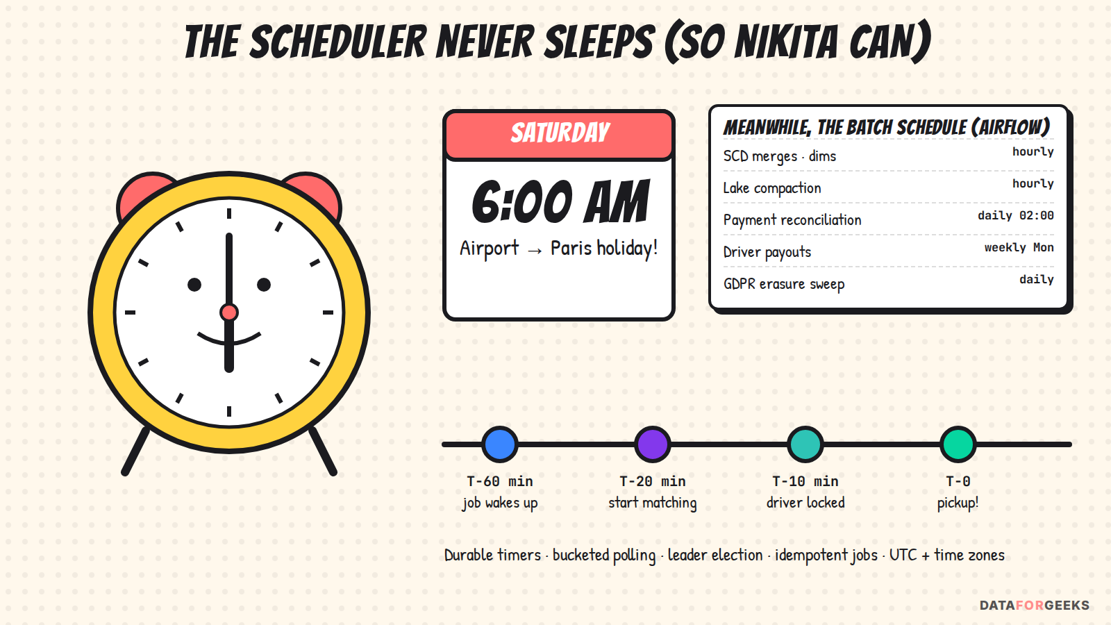
SCHEDULED → DISPATCHINGonly if the version matches), so two workers can’t dispatch the same ride. Delivery is at-least-once; processing is idempotent. - Timeline: T-60 the job wakes and checks supply forecasts; T-20 matching starts (with incentives if supply is thin); T-10 the driver is locked and Nikita is notified; T-0 pickup.
- Fallbacks: no driver by T-5 → widen the radius, raise incentives, notify the rider honestly with options.
Alternatives worth naming: durable workflow timers (Temporal, Step Functions) handle long waits well. Plain message-queue delays (e.g. SQS, which caps delivery delay at 15 minutes) don’t fit rides booked days ahead by themselves.
Batch orchestration (the data scheduler)
Overnight, Airflow (or Dagster) runs the platform’s housekeeping as DAGs with dependencies, retries, SLAs and alerting: hourly SCD merges and lake compaction, daily payment reconciliation at 02:00, weekly driver payouts, daily GDPR erasure sweeps, and nightly model retraining. Rules: tasks are idempotent (safe to re-run), partitioned by date (ds), backfill-friendly, and data-aware (start when the upstream partition lands, not just at 2:00 AM and hope).
THE INTERVIEWER ASKS
“The scheduler node dies at 5:59 AM. Does Nikita miss her flight?”
Strong answer: No. The worker’s lease expires within seconds, and another worker takes over its shards. Because the schedule is durable and the claim is a conditional state transition, the new worker sees the ride still in SCHEDULED (or a stale DISPATCHING past its timeout) and continues. Worst case a few seconds’ delay, never a lost or doubled dispatch. Monitoring: an alert on “rides overdue for dispatch > 0”.
THE INTERVIEWER ASKS
“Nikita schedules a ride in Paris for 2:30 AM on the night the clocks change. What happens?”
Strong answer: This is the classic DST trap. On spring-forward nights, 2:30 AM local time doesn’t exist; on fall-back nights, it happens twice. Store the rider’s intent as local time plus IANA zone (Europe/Paris), resolve it to UTC with explicit rules (e.g. “non-existent → shift forward; ambiguous → first occurrence”), and show the resolved time to the user. India doesn’t observe DST, so it’s easy to miss until you launch in a country that does.
THE INTERVIEWER ASKS
“Cron or an orchestrator for your data jobs?”
Strong answer: Cron runs commands. An orchestrator manages dependencies, retries, backfills, SLAs, lineage and visibility. For a few independent jobs, cron is fine. For a data platform where reconciliation depends on the ledger export, which depends on the lake compaction, use an orchestrator. Also mention ownership: every DAG has an owning team and an on-call rotation.
Chapter 14 · Monday, 10 AM: The analysts arrive
On Monday morning the analytics team shows up with questions. “Revenue by city and vehicle type last month?” “Average wait time for Gold-tier drivers?” “Is the new promo cannibalizing organic rides?” The operational model was built for writing one trip fast. They need a model built for reading millions of trips at once.
Nikhil switches hats and draws a dimensional model (Kimball-style star schema) in the gold layer:
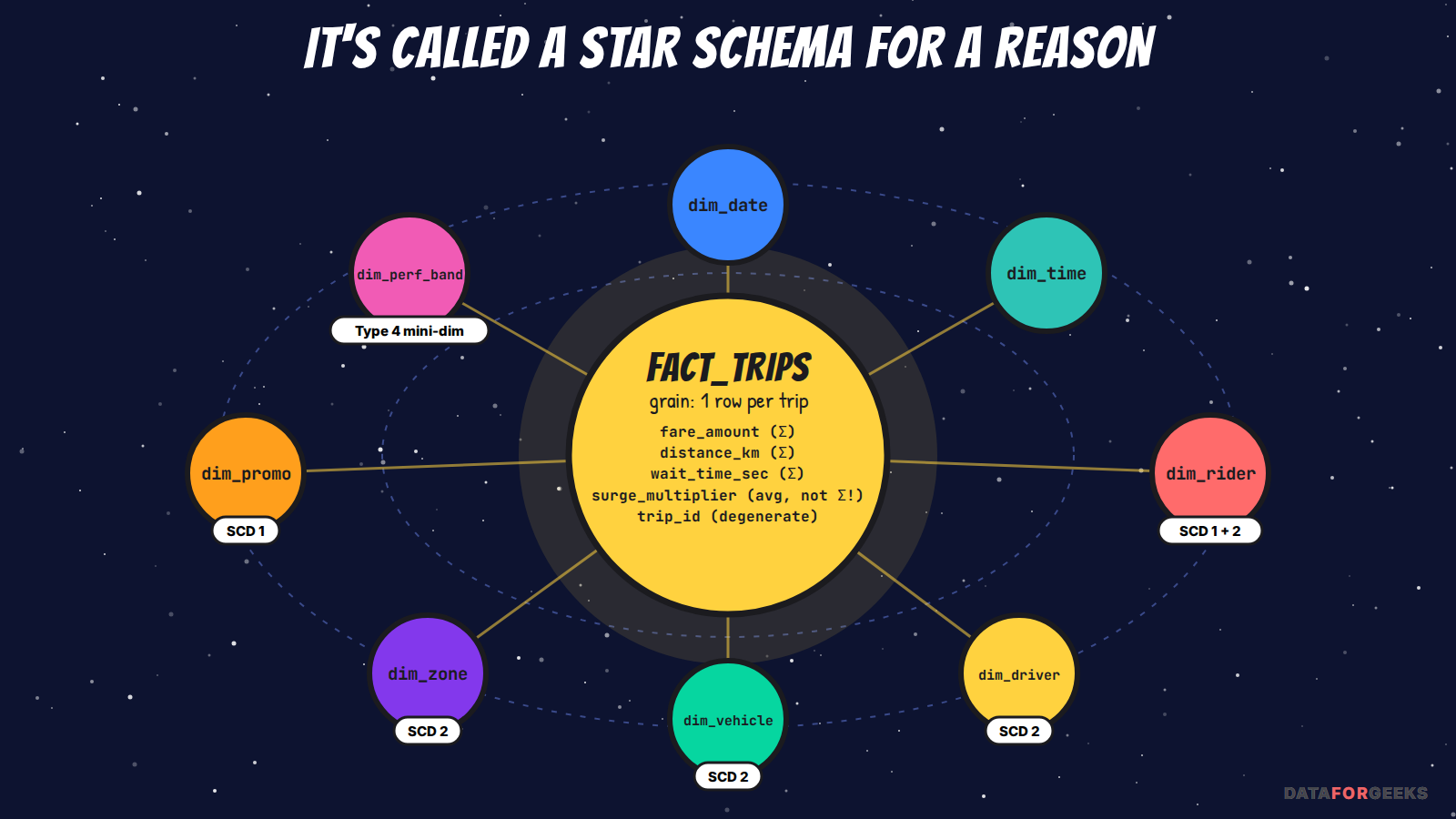
The facts (and their grain)
| Fact table | Type | Grain (one row per…) | Key measures |
|---|---|---|---|
fact_trips | Transaction | Trip (completed or cancelled) | fare, distance, duration, wait time, discount, tip; surge (non-additive) |
fact_trip_lifecycle | Accumulating snapshot | Trip, updated as milestones happen | requested_ts, accepted_ts, arrived_ts, started_ts, completed_ts, plus lags between them |
fact_trip_events | Transaction (event) | State transition | Counts, time since the previous event |
fact_driver_supply_hourly | Periodic snapshot | Driver × hour × zone | Online minutes, on-trip minutes, utilization |
fact_payments | Transaction | Ledger transaction | Amounts by account type, fees, refunds |
The dimensions
dim_date and dim_time (local and UTC variants), dim_rider, dim_driver, dim_vehicle, dim_zone (H3 cell → neighborhood → city → region, with boundaries that change over time), dim_promo, and a small dim_driver_perf_band mini-dimension. How each one keeps history is the next chapter, and it’s where many senior candidates slip.
THE INTERVIEWER ASKS
“What’s the grain of fact_trips?”
What they’re really testing: Kimball fundamentals. Grain is the first decision, and mixing grains is the classic error.
Strong answer: “One row per trip request that reached a terminal state (completed or cancelled).” Then defend it: per-event facts go in fact_trip_events, and per-hour driver facts go in a periodic snapshot. Never put per-trip and per-event rows in the same table, or sums double-count.
THE INTERVIEWER ASKS
“When would you use an accumulating snapshot instead of the event fact?”
Strong answer: When the business asks about pipeline durations: “time from request to accept”, “arrival to start”, “how many trips are stuck between accepted and started right now”. An accumulating snapshot has one row per trip with a column per milestone, updated as each happens, so those questions are simple column arithmetic instead of self-joins over the event table. It’s the funnel view; the event fact is the audit view.
THE INTERVIEWER ASKS
“Can I SUM(surge_multiplier)?”
Strong answer: No. It’s non-additive. Fare, distance and duration are additive. Ratings and multipliers need averages (ideally weighted: SUM(surge × base_fare) / SUM(base_fare)). Balances (e.g. wallet balance) are semi-additive: you can sum across accounts but not across time. Mentioning all three types shows you understand dimensional modeling properly.
THE INTERVIEWER ASKS
“‘Trips per day in Mumbai.’ Which day?”
Strong answer: The local day. Store event_ts in UTC, and also store local_date_key (computed with the city’s time zone) on the fact. Otherwise a trip at 1 AM IST lands on the previous UTC day, and daily reports quietly disagree with city ops. For a global rollup, state which convention you use.
Chapter 15 · Ravi upgrades his car (slowly changing dimensions)
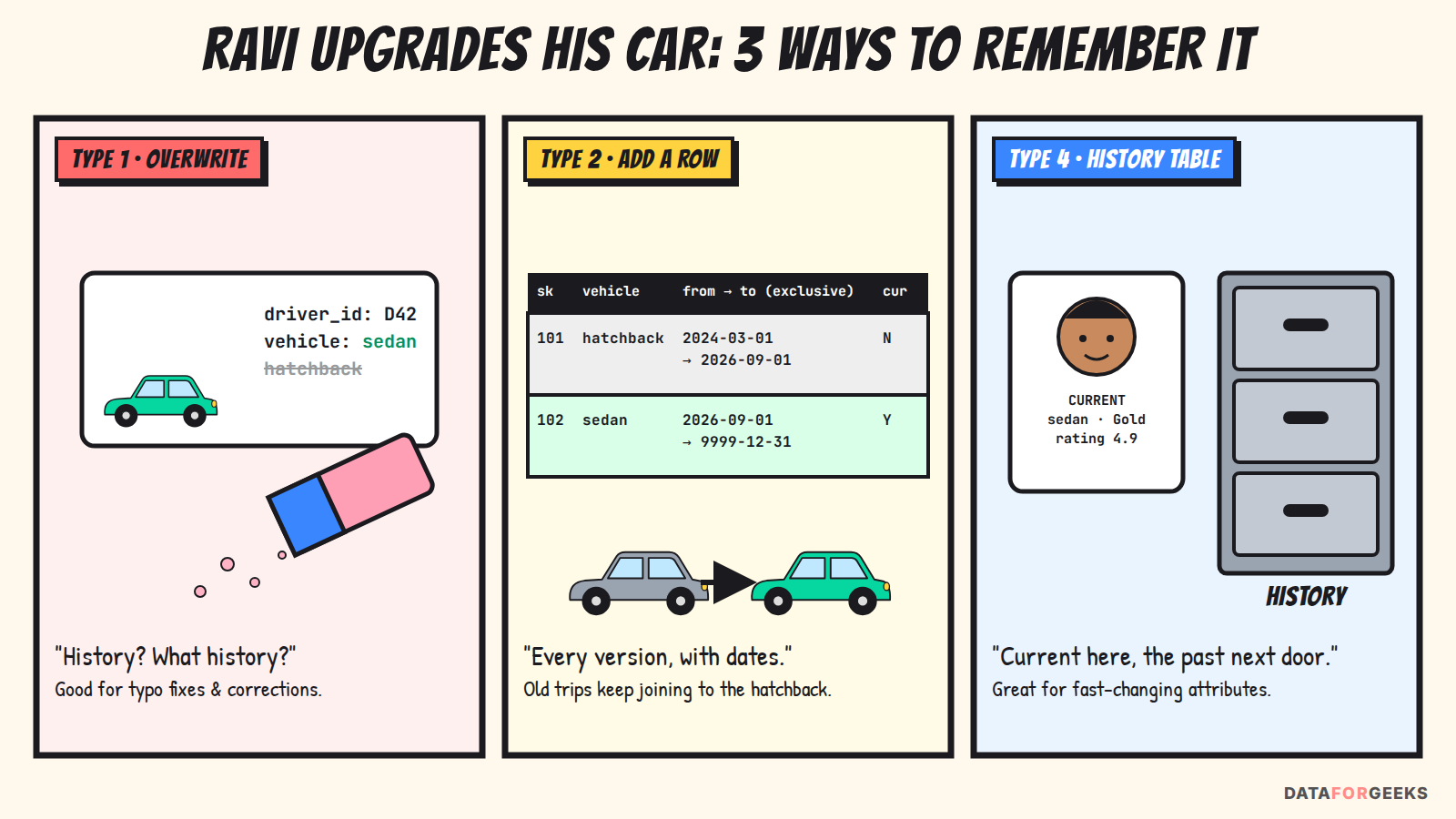
Good news for Ravi: on 1 September he upgraded from a hatchback to a sedan. The next quarterly review asks: “What was our revenue by vehicle type in August?” If dim_driver simply overwrote the vehicle, all of Ravi’s August hatchback trips now show up as sedan trips, and the numbers are wrong.
How a dimension handles change is the slowly changing dimension (SCD) type. It’s a design decision per attribute, not per table.
Type 1: overwrite (no history)
Replace the old value. Use it for corrections and attributes where history has no analytical value: a misspelled name, a corrected phone number, an email. It’s also what GDPR erasure needs (anonymize in place).
| driver_id | name | phone |
|---|---|---|
| D42 | Ravi Kumar |
Type 2: add a new row (full history)
Close the old row and insert a new one with a new surrogate key, effective_from / effective_to and an is_current flag. Facts store the surrogate key that was current when the trip happened, so August trips point to the hatchback row forever. (Here effective_to is exclusive: a row is valid while effective_from ≤ t < effective_to. Pick one convention and use it everywhere; off-by-one-day bugs in SCD joins are very common.)
| driver_sk | driver_id | vehicle_type | tier | home_city | effective_from | effective_to | is_current |
|---|---|---|---|---|---|---|---|
| 101 | D42 | hatchback | Silver | Bengaluru | 2024-03-01 | 2026-09-01 | N |
| 102 | D42 | sedan | Gold | Bengaluru | 2026-09-01 | 9999-12-31 | Y |
Use it for attributes that change reporting: vehicle type, driver tier, home city, commission plan, and zone boundaries in dim_zone (when a city redraws its surge zones, old trips must keep their old zone).
Type 4: separate history (and the “mini-dimension”)
For attributes that change very often, Type 2 would multiply rows. Ravi’s rating changes after every trip, so Type 2 would create hundreds of rows per driver. Type 4 moves volatility out of the main dimension. There are two common interpretations, and it’s worth saying both in an interview:
- History table:
dim_driverkeeps only current values (small, fast), anddim_driver_historyholds every past version for the rare question that needs it. - Mini-dimension (Kimball’s definition): put fast-changing attributes, banded, into a small separate dimension, e.g.
dim_driver_perf_band(rating_band '4.8–4.9', acceptance_band '90–95%', trips_band '1k–5k'). The fact row gets aperf_band_keyfor the band at trip time. There are only a few hundred band combinations, so there’s no row explosion, and history is still available through the facts.
Bonus types (in case they come up): Type 3 adds a “previous value” column (only one level of history, e.g. previous_city). Type 6 combines 1 + 2 + 3: Type 2 rows plus a current-value column overwritten on all rows, so you can report “as it was” and “as it is now” without a second join.
Which type for which attribute?
| Dimension · attribute | SCD type | Why |
|---|---|---|
| driver · name, phone, email | 1 | Corrections; PII; erasure-friendly |
| driver · vehicle_type, tier, home_city, commission_plan | 2 | Revenue and ops reporting depend on the value at trip time |
| driver · rating, acceptance rate, lifetime trips | 4 (mini-dimension, banded) | Changes every trip; banding avoids row explosion |
| rider · home_city, loyalty tier | 2 | Cohort and loyalty analysis |
| rider · name, phone, email | 1 | PII, corrections |
| zone · boundaries, surge-zone mapping | 2 | Historical trips keep historical zones |
| promo · description typo | 1 | No analytical value in the typo |
Building SCD Type 2 from the CDC stream
DynamoDB Streams feed driver changes into a driver_changes staging table. An hourly job merges them (Spark SQL on Delta/Iceberg shown; the same pattern works in Snowflake or BigQuery). First deduplicate driver_changes to the latest change per driver in the batch (or process changes in order), because MERGE fails when two source rows match the same target row:
MERGE INTO dim_driver AS t
USING (
  -- rows to INSERT as new versions (merge_key NULL never matches)
  SELECT NULL AS merge_key, c.* FROM driver_changes c
  JOIN dim_driver d ON d.driver_id = c.driver_id AND d.is_current
  WHERE d.row_hash <> c.row_hash
  UNION ALL
  -- rows used to CLOSE the current version, or insert brand-new drivers
  SELECT c.driver_id AS merge_key, c.* FROM driver_changes c
) AS s
ON t.driver_id = s.merge_key AND t.is_current
WHEN MATCHED AND t.row_hash <> s.row_hash THEN
  UPDATE SET is_current = false, effective_to = s.changed_at
WHEN NOT MATCHED THEN
  INSERT (driver_sk, driver_id, vehicle_type, tier, home_city, row_hash,
          effective_from, effective_to, is_current)
  VALUES (xxhash64(s.driver_id, s.changed_at), s.driver_id, s.vehicle_type, s.tier,
          s.home_city, s.row_hash, s.changed_at, TIMESTAMP '9999-12-31', true);
And the point-in-time answer to the quarterly question:
-- facts already carry driver_sk resolved at load time:
SELECT d.vehicle_type, SUM(f.fare_amount) AS revenue
FROM   fact_trips f JOIN dim_driver d ON f.driver_sk = d.driver_sk
WHERE  f.local_date_key BETWEEN 20260801 AND 20260831
GROUP  BY d.vehicle_type;

-- or, joining on the natural key + time range:
... JOIN dim_driver d ON f.driver_id = d.driver_id
     AND f.trip_ts >= d.effective_from AND f.trip_ts < d.effective_to
THE INTERVIEWER ASKS
“Ravi changed his car on 1 September. Show me August revenue by vehicle type.”
What they’re really testing: Whether you know SCD2 and point-in-time joins, not just the definition.
Strong answer: vehicle_type is Type 2 in dim_driver. Facts store the driver_sk that was current at trip time, so August trips join to the hatchback version. Also mention that the operational trips table already snapshotted vehicle_type at booking (Scene 4), which works as a cross-check.
THE INTERVIEWER ASKS
“Driver rating changes after every trip. Make it Type 2?”
Strong answer: No, that causes row explosion (millions of drivers × hundreds of versions) and slow joins. Use a Type 4 mini-dimension with bands, or treat rating as a measure in a periodic snapshot fact (fact_driver_daily.rating_avg). The exact rating at trip time is already on the trip row as driver_rating_snapshot.
THE INTERVIEWER ASKS
“A trip arrives referencing a driver who isn’t in dim_driver yet. What do you do?”
Strong answer: This is a late-arriving dimension (early-arriving fact). Don’t drop the fact and don’t block the pipeline. Insert an inferred member (a placeholder row with the natural key and “Unknown” attributes, flagged is_inferred), load the fact against it, and when the real dimension row arrives, update the inferred row in place (Type 1 style for that first version). Facts stay correct with no reload.
THE INTERVIEWER ASKS
“GDPR erasure with SCD Type 2: Léa has 6 historical rows. Now what?”
Strong answer: Type 2 multiplies PII, which is why the design separates PII into a Type 1 table (dim_rider_pii, one row per person) and keeps only non-PII attributes in the Type 2 dimension. Erasure then anonymizes one row, followed by lake snapshot expiry. If PII did leak into Type 2 history, anonymize every version and record the erasure in an audit log. This is where the compliance assumption from Scene 1 pays off.
THE INTERVIEWER ASKS
“Surrogate keys or natural keys in the warehouse?”
Strong answer: Surrogate keys for dimensions: they’re needed for Type 2 (one natural key, many versions), they insulate you from upstream key changes, and they join faster. Keep the natural key as an attribute for traceability. In lakehouses, deterministic hashes (e.g. hash(natural_key, effective_from)) avoid needing a central sequence.
Chapter 16 · The lightning round
With ten minutes left, the interviewer speeds up. These are quick questions that test breadth. One or two confident sentences each is enough.
| Question | Crisp answer |
|---|---|
| Shared rides (pool)? | A trip has many riders: add trip_riders(trip_id, rider_id, pickup, dropoff, fare_share, seq); matching becomes route insertion; fares split per rider. |
| Multi-stop trips? | trip_stops(trip_id, seq_no, location, arrived_at); new event types STOP_ARRIVED / STOP_DEPARTED. |
| Driver payouts? | Weekly batch from the ledger (driver:*.payable balances) → payout provider with idempotency keys → reversing entries on failure. |
| Fraud (GPS spoofing, fake trips)? | Real-time features from location logs (impossible speed, teleporting), device fingerprints, graph links between accounts; score in the stream, act before payout. |
| Kafka schema changes? | Schema registry with Avro/Protobuf; backward-compatible changes only (add optional fields); CI checks compatibility. |
| Replay last Tuesday? | Kafka retention for recent days, bronze lake tables for older; idempotent consumers; Iceberg time travel to compare before and after. |
| Data retention? | GPS: 30 days in OLTP (TTL) → lake, compacted, cold tier after 90 days; trips and ledger: legally required years; PII: minimal and purpose-bound. |
| Security? | TLS everywhere, KMS encryption with per-region keys, tokenized payment data (never store raw card numbers; PCI scope minimized), column-level access in the lake, audit logs of access. |
| Testing at scale? | Contract tests between services, load tests with replayed traffic, chaos/game days (kill Redis, partition a region), shadow traffic for new matching algorithms. |
| Rolling out a new matching algorithm? | Feature flag + A/B by city or cell; guardrail metrics (match rate, cancellations, ETA error); automatic rollback on SLO burn. |
| Cost? | TTLs and tiering for GPS, on-demand vs provisioned capacity by traffic shape, compaction to fight small files, right-sized Redis (the napkin says ~200 MB of live state, so don’t buy terabytes). |
| Rider and driver safety? | SOS and trip-sharing features are P0 (never shed), route-deviation detection runs on the live location stream, and safety events get their own audit trail and restricted access. |
| Where does the feature store fit? | Streaming features (Flink) for online serving at low latency, batch features from the lake for training; same definitions for both, to avoid training/serving skew. |
Epilogue: Back in the interview room
Nikhil looks at the clock: 44 minutes. The whiteboard shows one ride, followed from tap to payment and then into the warehouse, with every component placed where it was needed.
He summarizes the whole journey in one line, the same real-time workflow he started with:
Rider requests → gateway (auth, rate limit) → booking service queries Redis → match driver (conditional write) → update Redis + write DynamoDB → notify → track location via stream → complete → pay (idempotent ledger) → archive to lake → dashboards, analytics and ML.
The interviewer caps the marker and says, “Most people give me 47 tables. You gave me a system.”
The practice session moves on to the next topic. Later that evening Nikhil and Nikita head out for dinner, and the cab is booked in under 400 milliseconds, of course.
Here’s everything you might get asked, in bingo form. Screenshot it before your next loop.
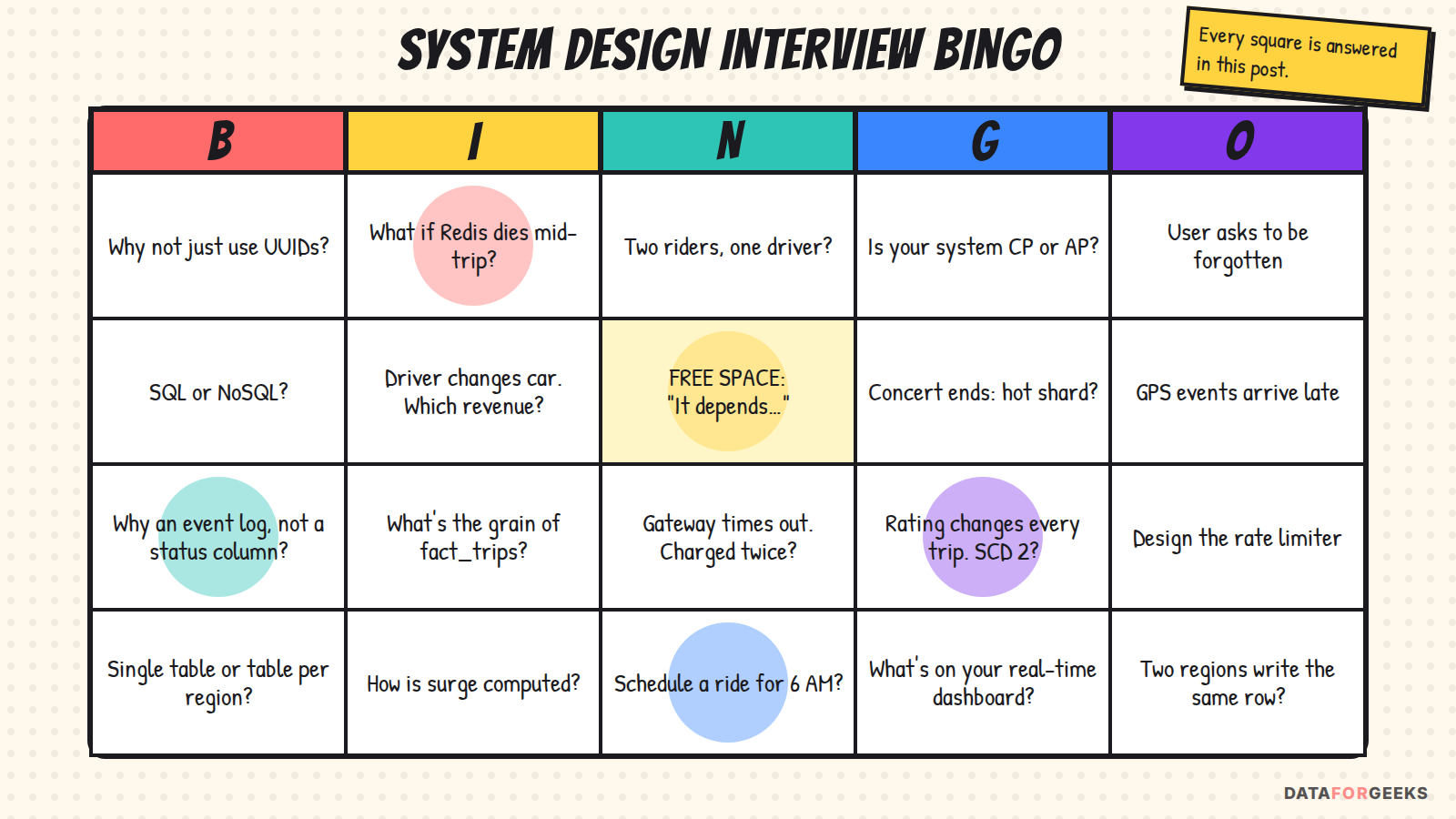
The cheat sheet
| If they ask… | Say this in one breath | Where |
|---|---|---|
| How will you approach this? | Requirements → napkin → front door and APIs → data model → scale and failure → analytics and evolution | Scene 1 |
| How much data? | 230 trips/s, 250K pings/s, ~2 TB/day GPS, ~200 MB live state: history is huge, “now” is tiny | Scene 2 |
| What does the gateway do? | Auth, rate limits, validation, routing, idempotency keys, tracing; no business logic | Scene 3 |
| Design a rate limiter | Token bucket in Redis via atomic Lua, layered limits, 429 + Retry-After, fail open or closed per endpoint | Scene 3 |
| NYE 20× traffic? | Pre-scale, priority shedding, surge, degrade tracking, cell isolation | Scene 3 |
| SQL or NoSQL? | Per workload: DynamoDB for hot OLTP, Postgres for the ledger, lake for history | Scene 1, Ch 10 |
| Why not query the DB for drivers? | High-churn, read-heavy geo data belongs in Redis with TTLs | Ch 1 |
| Two riders, one driver? | Conditional write on the source of truth; the loser retries the next driver | Ch 2 |
| Dual write fails halfway? | DB first, cache second, idempotent writes, outbox/CDC repair | Ch 2 |
| CP or AP? | Per operation: CP for assignment and money, AP for location and analytics; PACELC | Ch 3 |
| Hot shard at the stadium? | H3 cells, split to finer resolution, salting, caching and coalescing, pre-warm | Ch 4 |
| Reshard without downtime? | Logical shards; dual-write → backfill → verify → shadow-read → cut over | Ch 4 |
| Why an event log? | History, replay, audits, process mining; the status column only keeps the last state | Ch 5 |
| Single table or per region? | Single table with region_id unless the law requires separation | Ch 6 |
| Region goes down? | RPO/RTO per data class, replicated standby, practiced failover | Ch 6 |
| Redis dies? | Not the source of truth; fall back to DB, prevent stampede, geo index self-heals | Ch 7 |
| Retry storm? | Backoff + jitter, retry budgets, one retry layer, breakers, shedding | Ch 8 |
| Poison message? | Bounded retries → DLQ → alert → fix → replay | Ch 8 |
| Why not UUIDs? | Not sortable; Snowflake/ULID/UUIDv7 give time order without coordination | Ch 9 |
| Gateway timeout, charged twice? | Unknown ≠ failed; same idempotency key, status query, reconciliation | Ch 10 |
| Late GPS events? | Event time, watermarks, date partitions, idempotent backfills | Ch 11 |
| Right to be forgotten? | No PII in events; Type 1 PII table; lakehouse deletes + snapshot expiry; crypto-shredding | Ch 11, 15 |
| Know before users do? | Business SLIs (match rate, time to match) with burn-rate alerts, plus traces keyed by trip_id | Ch 12 |
| Dashboard ≠ finance? | Event vs processing time, time zones, dedupe, definitions; semantic layer | Ch 12 |
| Scheduled rides? | Durable schedule, bucketed polling with leases, conditional claim, UTC + IANA zone | Ch 13 |
| Grain of fact_trips? | One row per trip in a terminal state; events and snapshots in their own facts | Ch 14 |
| Driver changed car? | SCD Type 2 with surrogate keys and a point-in-time join | Ch 15 |
| Rating changes every trip? | Type 4 banded mini-dimension, or a measure in a snapshot fact | Ch 15 |
What makes this a strong answer
It isn’t about knowing more tools. Anyone can list Redis, Kafka and DynamoDB. What makes the difference:
- You drive. You set the agenda, manage the time and invite the interviewer to steer.
- You tell a story. Following one ride gives the interviewer a map of your thinking, which a list of tables doesn’t.
- You explain why. Every component is tied to a moment in the ride, a number from the napkin, and a trade-off you chose.
- You bring up failure yourself. Races, outages, retry storms, clock skew, hot shards and late data come up before the interviewer asks.
- You think in operations. SLOs, dashboards, runbooks, rollouts and cost are part of the design.
- You design for later. Event logs, region keys, sortable IDs and SCDs make next year’s questions cheap to answer.
Nikita got home in 27 minutes. Nikhil’s whiteboard took 44. With this design, you can give your answer in 45.
Found this useful? Share it with someone who has a system design round coming up. Tell us in the comments which bingo square you’ve been asked, and which one caught you out.